Exploring Topology Control in Networks
Understand different proximity graphs like Gabriel Graph and Delaunay Triangulation used in Topology Control for network connectivity and energy conservation.

Exploring Topology Control in Networks
E N D
Presentation Transcript
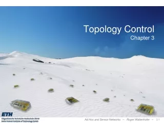
Topology ControlChapter 3 TexPoint fonts used in EMF. Read the TexPoint manual before you delete this box.: AAAA
Inventory Tracking (Cargo Tracking) • Current tracking systems require line-of-sight to satellite. • Count and locate containers • Search containers for specific item • Monitor accelerometer for sudden motion • Monitor light sensor for unauthorized entry into container
Rating • Area maturity • Practical importance • Theory appeal First steps Text book No apps Mission critical Boooooooring Exciting
Overview – Topology Control • Proximity Graphs: Gabriel Graph et al. • Practical Topology Control: XTC • Interference
Topology Control • Drop long-range neighbors: Reduces interference and energy! • But still stay connected (or even spanner)
Topology Control as a Trade-Off Topology Control Network ConnectivitySpanner Property Conserve EnergyReduce Interference Sparse Graph, Low Degree Planarity Symmetric Links Less Dynamics dTC(u,v) · c ¢ d(u,v)
Spanners • Let the distance of a path from node u to node v, denoted as d(u,v), be the sum of the Euclidean distances of the links of the shortest path. • Writing d(u,v)p is short for taking each link distance to the power of p, again summing up over all links. • Basic idea: S is spanner of graph G if S is a subgraph of G that has certain properties for all pairs of nodes, e.g. • Geometric spanner: dS(u,v) ≤ c¢dG(u,v) • Power spanner: dS(u,v)α ≤ c¢dG(u,v)α, for path loss exponent α • Weak spanner: path of S from u to v within disk of diameter c¢dG(u,v) • Hop spanner: dS(u,v)0 ≤ c¢dG(u,v)0 • Additive hop spanner: dS(u,v)0 ≤ dG(u,v)0 + c • (α, β) spanner: dS(u,v)0 ≤ α¢dG(u,v)0 + β • The stretch can be defined as maximum ratio dS/dG
Gabriel Graph • Let disk(u,v) be a disk with diameter (u,v)that is determined by the two points u,v. • The Gabriel Graph GG(V) is defined as an undirected graph (with E being a set of undirected edges). There is an edge between two nodes u,v iff the disk(u,v) including boundary contains no other points. • As we will see the Gabriel Graph has interesting properties. v disk(u,v) u
Delaunay Triangulation • Let disk(u,v,w) be a disk defined bythe three points u,v,w. • The Delaunay Triangulation (Graph) DT(V) is defined as an undirected graph (with E being a set of undirected edges). There is a triangle of edges between three nodes u,v,wiff the disk(u,v,w) contains no other points. • The Delaunay Triangulation is thedual of the Voronoi diagram, andwidely used in various CS areas • the DT is planar • the DT is a geometric spanner v disk(u,v,w) w u
Other Proximity Graphs • Relative Neighborhood Graph RNG(V) • An edge e = (u,v) is in the RNG(V) iffthere is no node w in the “lune” of (u,v), i.e., no noe with with(u,w) < (u,v) and (v,w) < (u,v). • Minimum Spanning Tree MST(V) • A subset of E of G of minimumweightwhichforms a tree on V. u v
Properties of Proximity Graphs • Theorem 1:MST µ RNG µ GG µ DT • Corollary:Since the MST is connected and the DT is planar, all the graphs in Theorem 1 are connected and planar. • Theorem 2:The Gabriel Graph is a power spanner (for path loss exponent ¸ 2). So is GG Å UDG. • Remaining issue: either high degree (RNG and up), and/or no spanner (RNG and down). There is an extensive and ongoing search for “Swiss Army Knife” topology control algorithms.
More Proximity Graphs • -Skeleton • Disk diameters are ¢d(u,v), going through u resp. v • Generalizing GG ( = 1) and RNG ( = 2) • Yao-Graph • Each node partitions directions in k cones and then connects to theclosest node in each cone • Cone-Based Graph • Dynamic version of the YaoGraph. Neighbors are visitedin order of their distance, and used only if they covernot yet covered angle
Lightweight Topology Control • Topology Control commonly assumes that the node positions are known. What if we do not have access to position information?
Each node produces “ranking” of neighbors. Examples Distance (closest) Energy (lowest) Link quality (best) Mustbesymmetric! Not necessarily depending on explicit positions Nodes exchange rankings with neighbors XTC: Lightweight Topology Control without Geometry D C G B A 1. C 2. E 3. B 4. F 5. D 6. G E F
Each node locally goes through all neighbors in order of their ranking If the candidate (current neighbor) ranks any of your already processed neighbors higher than yourself, then you do not need to connect to the candidate. XTC Algorithm (Part 2) 2. C 4. G 5. A 3. B 4. A 6. G 8. D 4. B 6. A 7. C D C G 7. A 8. C 9. E B 1. F 3. A 6. D A 1. C 2. E 3. B 4. F 5. D 6. G E F 3. E 7. A
XTC Analysis (Part 1) • Symmetry: A node u wants a node v as a neighbor if and only if v wants u. • Proof: • Assume 1) u v and 2) u v • Assumption 2) 9w: (i) w Áv u and (ii) w Áu v In node u’s neighborlist, w is better than v Contradicts Assumption 1)
XTC Analysis (Part 1) • Symmetry: A node u wants a node v as a neighbor if and only if v wants u. • Connectivity: If two nodes are connected originally, they will stay so (easy to show if rankings are based on symmetric link-weights). • If the ranking is energy or link quality based, then XTC will choose a topology that routes around walls and obstacles.
XTC Analysis (Part 2) • If the given graph is a Unit Disk Graph (no obstacles, nodes homogeneous, but not necessarily uniformly distributed), then … • The degree of each node is at most 6. • The topology is planar. • The graph is a subgraph of the RNG. • Relative Neighborhood Graph RNG(V): • An edge e = (u,v) is in the RNG(V) iffthere is no node w with (u,w) < (u,v) and (v,w) < (u,v). u v
XTC Average-Case Unit Disk Graph XTC
XTC Average-Case (Degrees) v u UDG max UDG avg GG max GG avg XTC max XTC avg
XTC Average-Case (Stretch Factor) XTC vs. UDG – Geometric GG vs. UDG – Geometric XTC vs. UDG – Power GG vs. UDG –Power
Implementing XTC, e.g. on mica2 motes • Idea: • XTC chooses the reliable links • The quality measure is a moving average of the received packet ratio • Source routing: route discovery (flooding) over these reliable links only • (black: using all links, grey: with XTC)
Topology Control as a Trade-Off Topology Control Network ConnectivitySpanner Property Conserve Energy Reduce Interference Sparse Graph, Low Degree Planarity Symmetric Links Less Dynamics Really?!?
What is Interference? Exact size of interference rangedoes not change the results • Problem statement • We want to minimize maximum interference • At the same time topology must be connected or spanner Link-based Interference Model Node-based Interference Model Interference 8 Interference 2 „How many nodes are affected by communication over a given link?“ „By how many other nodes can a given network node be disturbed?“
Low Node Degree Topology Control? Low node degree does not necessarily imply low interference: Very low node degree but huge interference
Let’s Study the Following Topology! …from a worst-case perspective
Topology Control Algorithms Produce… • All known topology control algorithms (with symmetric edges) include the nearest neighbor forest as a subgraph and produce something like this: • The interference of this graph is (n)!
But Interference… • Interference does not need to be high… • This topology has interference O(1)!!
v u 5 9 9 3 8 4 2 8 Link-based Interference Model There is no local algorithmthat can find a goodinterference topology The optimal topologywill not be planar
3 5 4 6 3 10 5 2 4 3 11 9 4 11 9 2 8 7 8 3 7 8 2 5 6 3 7 4 4 3 3 2 4 8 Link-based Interference Model • LIFE (Low Interference Forest Establisher) • Preserves Graph Connectivity LIFE • Attribute interference values as weights to edges • Compute minimum spanning tree/forest (Kruskal’s algorithm) Interference 4 LIFE constructs a minimum- interference forest
Average-Case Interference: Preserve Connectivity UDG GG RNG LIFE
2 1 4 8 Node-based Interference Model • Already 1-dimensional node distributions seem to yield inherently high interference... Connecting linearly results in interference O(n) • ...but the exponential node chain can be connected in a better way
Interference Node-based Interference Model • Already 1-dimensional node distributions seem to yield inherently high interference... Connecting linearly results in interference O(n) • ...but the exponential node chain can be connected in a better way Matches an existing lower bound
Node-based Interference Model • Arbitrary distributed nodes in one dimension • Approximation algorithm with approximation ratio in O( ) • Two-dimensional node distributions • Simple randomized algorithm resulting in interference O( ) • Can be improved to O(√n)
Open problem • On the theory side there are quite a few open problems. Even the simplest questions of the node-based interference model are open: • We are given n nodes (points) in the plane, in arbitrary (worst-case) position. You must connect the nodes by a spanning tree. The neighbors of a node are the direct neighbors in the spanning tree. Now draw a circle around each node, centered at the node, with the radius being the minimal radius such that all the nodes’ neighbors are included in the circle. The interference of a node u is defined as the number of circles that include the node u. The interference of the graph is the maximum node interference. We are interested to construct the spanning tree in a way that minimizes the interference. Many questions are open: Is this problem in P, or is it NP-complete? Is there a good approximation algorithm? Etc.