Sideband Deconvolution
Sideband Deconvolution. Outline. What is sideband deconvolution and why it is necessary for HIFI data? General description of the algorithm Implementation within HIPE Workflow for spectral scans. Heterodyne observations.

Sideband Deconvolution
E N D
Presentation Transcript
Outline • What is sideband deconvolution and why it is necessary for HIFI data? • General description of the algorithm • Implementation within HIPE • Workflow for spectral scans
Heterodyne observations • Detectors are not able to directly measure flux at the frequencies of interest. But by mixing the signal from the sky with a local oscillator, we `downconvert’ the frequency. • cos(ω)cos(νLO)=0.5[ cos(ω-νLO) + cos(ω+νLO) ] • When ω is the entire, unfiltered sky frequency, you end up being sensitive to TWO bandpasses. (cos(ν) = cos(-ν))
Heterodyne observations νLO USB LSB What is being measured -> Sky frequency How it looks when collected-> IF
Heterodyne observations νLO USB LSB What is being measured -> Sky frequency How it looks when collected-> IF
Heterodyne observations νLO USB LSB What is being measured -> Sky frequency How it looks when collected-> IF
Heterodyne observations νLO USB LSB What is being measured -> Sky frequency How it looks when collected-> IF
Heterodyne observations νLO USB LSB What is being measured -> Sky frequency How it looks when collected-> IF
Heterodyne observations νLO USB LSB What is being measured -> Sky frequency How it looks when collected-> IF
Heterodyne observations νLO USB LSB What is being measured -> Sky frequency How it looks when collected-> IF
Heterodyne observations νLO USB LSB What is being measured -> Sky frequency How it looks when collected-> IF
Heterodyne observations νLO USB LSB What is being measured -> Sky frequency How it looks when collected-> IF
Heterodyne observations νLO USB LSB What is being measured -> Sky frequency How it looks when collected-> IF
Heterodyne observations νLO USB LSB What is being measured -> Sky frequency How it looks when collected-> IF
Heterodyne observations νLO USB LSB What is being measured -> Sky frequency How it looks when collected-> IF
Heterodyne observations LSB + USB = DSB LO • Lower sideband spectrum is reversed and added • Two frequency scales result in the DSB result • The lines may blend but they can be recovered (deconvolved) • The continuum levels add (double) in the DSB • The continuum slope is flattened but may be recovered (deconvolved) • The noise adds in quadrature , increasing as sqrt(2)
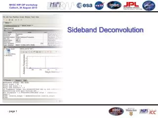
Sideband Deconvolution • The problem is the following: Given a collection of double sideband data taken over several LO tunings, how do we recover the original ‘sky’ spectrum? • Comito & Schilke(2002) provide an algorithm which has been successfully employed with ground based heterodynes. • Has been implemented in CLASS + X-CLASS (Fortran based) but was converted to JAVA for use within HIPE. Upgrades to the algorithm have been almost exclusively within HIPE.
Deconvolution Algorithm • Start with a guess of the answer – a model with no assumptions for the SSB spectrum – flat • "Observe it" – using knowledge of the instrument • compare the observations of the model with the real observations • compute a chi square and a delta (differential) chi-square • each model "spectral channel" was in part responsible for some of the chi square change • follow the slope of the chi square downward (it's partial derivitivew.r.t. the channel flux (and optionally the sideband gain) • new downward steps always move at right angles to previous ones in the Conjugate Gradient Method • Stop, when solution converges asymptotically, as defined by the "tolerance" It’s iterative
doDeconvolution caveats • Iteration requires that the data make sense. • Sufficient redundancy (~100% of the time) • No spurs • Compatible baselines • No (or well behaved) standing waves Most work is done before deconvolution
Decon GUI Some features not recommended at all (may be deprecated in a later release) Some features not used very often
Demos • Basic deconvolution • How unflagged spurs affect decon output • Carefully flagging bad data improves result • The diagnostic mode (advanced) • Ghosts and ‘Bright Lines’