Hierarchical Affinity Propagation
Hierarchical Affinity Propagation. Inmar E. Givoni , Clement Chung, Brendan J. Frey. outline. A Binary Model for Affinity Propagation Hierarchical Affinity Propagation Experiments. A Binary Model for Affinity Propagation.

Hierarchical Affinity Propagation
E N D
Presentation Transcript
Hierarchical Affinity Propagation Inmar E. Givoni, Clement Chung, Brendan J. Frey
outline • A Binary Model for Affinity Propagation • Hierarchical Affinity Propagation • Experiments
A Binary Model for Affinity Propagation AP was originally derived as an instance of the max-product (belief propagation) algorithm in a loopy factor graph. What’s factor graph? • Definition: A factor graphis a bipartite graph that expresses the structure of the factorization. A factor graph has a variable nodefor each variable , a factor nodefor each local function , and an edge-connecting variable node to factor node if and only if is an argument of.
Definition:所谓factor graph(因子图),就是对函数因子分解的表示图,一般内含两种节点,变量节点和函数节点。我们知道,一个全局函数能够分解为多个局部函数的积,因式分解就行了,这些局部函数和对应的变量就能体现在因子上。 Eg是一个五个变量的函数,假设g可以表达成: A factor graph for the product
The Max-Sum Update Rules 变量节点发给函数节点的消息:是变量节点收到其他与之关联的函数节点发来的消息的和。 where the notation ne(x)\ f is used to indicate the set of variable node x’s neighbors excluding function node f .
函数节点发给变量节点的消息:是函数节点的值和其他变量节点发给它的消息累加和的最大值。函数节点发给变量节点的消息:是函数节点的值和其他变量节点发给它的消息累加和的最大值。 • ne( f )\x is used to indicate the set of function node f ’s neighbors excluding variable node x.
A binary variable model for affinity propagation • ci j = 1 if the exemplar for point iis point j. • ,,:the I function nodes, in every row iof the grid, exactly one ci j , j ∈ {1, . . . , N}, variable must be set to 1. The E function nodes enforce the exemplar consistency constraints; in every column j, the set of ci j , i∈ {1, . . . , N}, variables set to 1 indicates all the points that have chosen point j as their exemplar.
We derive the scalar message updates in the binary variable AP model. Recall the max-sum message update rules. • The scalar message difference βi j (1) − βi j (0) is denoted by βi j . Similar notation is used for α, ρ, and η. In what follows, for each message we calculate its value for each setting of the binary variable and then take the difference.
The αi j messages are identical to the AP availability messages a(i, j),and the ρi j messages are identical to the AP responsibility messages r (i, j).Thus, we have recovered the original affinity propagation updates.
Hierarchical Affinity Propagation • Goal: to solve the hierarchical clustering problem. • What’s hierarchical clustering ? 层次聚类算法与之前所讲的聚类有很大不同,它不再产生单一聚类,而是产生一个聚类层次。说白了就是一棵层次树。 层次聚类算法可分为凝聚(agglomerative,自底向上)和分裂(divisive,自顶向下)两种。自底向上,一开始,每个数据点各自为一个类别,然后每一次迭代选取距离最近的两个类别,把他们合并,直到最后只剩下一个类别为止,至此一棵树构造完成。自顶向下与之相反过程。
Model • Goal: We propose a hierarchical exemplar based clustering objective function in terms of a high-order factor-graph, and we derive an efficient approximate loopy max-sum algorithms. • We wish to find a set of L consecutive layers of clustering, where the points to be clustered in layer l are constrained to be in the exemplar set of layer l-1.
(a) HAP factor-graph, a single layer of the standard AP model is shown in the dotted square. (b) HAP messages.
Differences 1.The main difference compared to the at representation is manifested in the functions: if point i is not chosen as an exemplar at layer l-1, (i.e. if = 0), then point i will not be clustered at layer l. Alternatively, if point i is chosen as an exemplar at layer l-1, it must choose an exemplar at layer l.
2 • We note the 1ij messages passed in the first layer and the Lijmessages passed in the top-most layer are identical to the standard AP messages for an AP layer.
Experiments 2D synthetic data Analysis of Synthetic HIV Sequences
Figure : 2D synthetic data: comparison of objective Eq. (8) achieved by HAP and its greedy counterpart (Greedy). Top:Medianpercent improvement of HAP over Greedy for a given number of layers used. Bottom: Scatter plots of the net similarity achieved by HAP v.s. Greedy. Experiments for which HAP obtains better results than Greedy are below the line. Total percent of settings where HAP outperforms Greedy is reported in the inset. Color in scatter-plot indicates the number of layers.
First, we plotted precision v.s. recall for various clustering settings • Synthetic HIV data: precision-recall for HAP, Greedy, HKMC and HKMeans applied to the problem of identifying ancestral sequences from a set of 867 synthetic HIV sequences. For HKMC and HKMeans, we only plot the best precision obtained for each unique recall value.
Synthetic HIV data: distribution of Rand index for different experiments using HAP and Greedy. A higher Rand index indicates the solution better resembles the ground truth. Experiments for which HAP obtains better results than Greedy are below the line. The percentage of solutions that identified the correct single ancestor sequence at the top layer (layer 4) is also reported.