Download

1 / 93
990 likes | 1.58k Vues
7. Integration by Parts Integration Using Tables of Integrals Numerical Integration Improper Integrals Applications of Calculus to Probability. Additional Topics in Integration. 7.1. Integration by Parts. The Method of Integration by Parts. Integration by parts formula. Example.

E N D
7 • Integration by Parts • Integration Using Tables of Integrals • Numerical Integration • Improper Integrals • Applications of Calculus to Probability Additional Topics in Integration
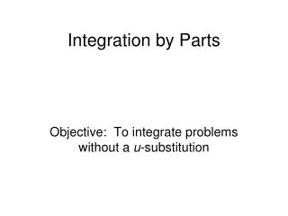
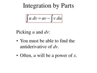
7.1 Integration by Parts
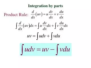
The Method of Integration by Parts • Integration by parts formula
Example • Evaluate Solution • Let u = x and dv = ex dx • So that du = dx and v = ex • Therefore, Example 1, page 484
Guidelines for Integration by Parts • Choose u an dv so that • du is simpler than u. • dv is easyto integrate.
Example • Evaluate Solution • Let u =lnx and dv = xdx • So that and • Therefore, Example 2, page 485
Example • Evaluate Solution • Let u = xex and • So that and • Therefore, Example 3, page 486
Example • Evaluate Solution • Let u = x2 and dv = ex dx • So that du = 2xdx and v = ex • Therefore, (From first example) Example 4, page 486
Applied Example: Oil Production • The estimated rate at which oil will be produced from an oil well tyears after production has begun is given by thousand barrels per year. • Find an expression that describes the total production of oil at the end of yeart. Applied Example 5, page 487
Applied Example: Oil Production Solution • Let T(t) denote the total production of oil from the well at the end of yeart (t 0). • Then, the rate of oil production will be given by T′(t) thousand barrels per year. • Thus, • So, Applied Example 5, page 487
Applied Example: Oil Production Solution • Use integration by parts to evaluate the integral. • Let and • So that and • Therefore, Applied Example 5, page 487
Applied Example: Oil Production Solution • To determine the value of C, note that the total quantity of oil produced at the end of year0 is nil, so T(0) = 0. • This gives, • Thus, the required production function is given by Applied Example 5, page 487
7.2 Integration Using Tables of Integrals
A Table of Integrals • We have covered several techniques for finding the antiderivatives of functions. • There are many more such techniques and extensive integration formulas have been developed for them. • You can find a table of integrals on pages491 and 492 of the text that include some such formulas for your benefit. • We will now consider some examples that illustrate how this table can be used to evaluate an integral.
Examples • Use the table of integrals to find Solution • We first rewrite • Since is of the form , with a = 3, b = 1, and u = x, we use Formula (5), obtaining Example 1, page 493
Examples • Use the table of integrals to find Solution • We first rewrite3 as , so that has the form with and u = x. • Using Formula (8), obtaining Example 2, page 493
Examples • Use the table of integrals to find Solution • We can use Formula (24), • Letting n = 2, a = – ½, and u = x, we have Example 5, page 494
Examples • Use the table of integrals to find Solution • We have • Using Formula (24) again, with n = 1, a = – ½, and u = x, we get Example 5, page 494
Applied Example: Mortgage Rates • A study prepared for the National Association of realtors estimated that the mortgage rate over the next tmonths will be percent per year. • If the prediction holds true, what will be the average mortgage rate over the 12months? Applied Example 6, page 495
Applied Example: Mortgage Rates Solution • The average mortgage rate over the next 12months will be given by Applied Example 6, page 495
Applied Example: Mortgage Rates Solution • We have • Use Formula (1) to evaluate the first integral or approximately 6.99%per year. Applied Example 6, page 495
7.3 Numerical Integration
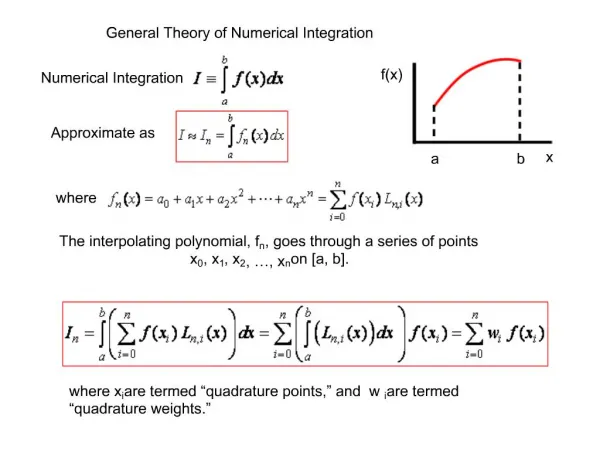
Approximating Definite Integrals • Sometimes, it is necessary to evaluate definite integrals based on empirical data where there is no algebraic rule defining the integrand. • Other situations also arise in which an integrable function has an antiderivative that cannot be found in terms of elementary functions. Examples of these are • Riemann sums provide us with a good approximation of a definite integral, but there are better techniques and formulas, called quadrature formulas, that allow a more efficient way of computing approximate values of definite integrals.
The Trapezoidal Rule • Consider the problem of finding the area under the curve of f(x) for the interval [a, b]: y R x a b
The Trapezoidal Rule • The trapezoidal rule is based on the notion of dividing the area to be evaluated into trapezoids that approximate the area under the curve: y R1 R2 R3 R4 R5 R6 x a b
The Trapezoidal Rule • The incrementsx used for each trapezoid are obtained by dividing the interval into nequal segments (in our example n = 6): y x R1 R2 R3 R4 R5 R6 x a b
The Trapezoidal Rule • The area of each trapezoid is calculated by multiplying its base, x, by its average height: y x f(x0) R1 f(x1) x x0 = a x1 b
The Trapezoidal Rule • The area of each trapezoid is calculated by multiplying its base, x, by its average height: y x f(x1) R2 f(x2) x a x1 x2 b
The Trapezoidal Rule • The area of each trapezoid is calculated by multiplying its base, x, by its average height: y f(x2) R3 f(x3) x a x2 x3 b
The Trapezoidal Rule • The area of each trapezoid is calculated by multiplying its base, x, by its average height: y R4 f(x3) f(x4) x a x3 b x4
The Trapezoidal Rule • The area of each trapezoid is calculated by multiplying its base, x, by its average height: y R5 f(x4) f(x5) x a b x4 x5
The Trapezoidal Rule • The area of each trapezoid is calculated by multiplying its base, x, by its average height: y R6 f(x5) f(x6) x a b = x6 x5
The Trapezoidal Rule • Adding the areasR1 through Rn (n = 6 in this case) of the trapezoids gives an approximation of the desired area of the region R: y R1 R2 R3 R4 R5 R6 x a b
The Trapezoidal Rule • Adding the areasR1 through Rn of the trapezoids yields the following rule: • Trapezoidal Rue
Example • Approximate the value of using the trapezoidal rule with n = 10. • Compare this result with the exact value of the integral. Solution • Here, a = 1, b = 2, an n = 10, so and x0 = 1, x1 = 1.1, x2 = 1.2, x3 = 1.3, … , x9 = 1.9, x10 = 1.10. • The trapezoidal rule yields Example 1, page 500
Example • Approximate the value of using the trapezoidal rule with n = 10. • Compare this result with the exact value of the integral. Solution • By computing the actual value of the integral we get • Thus the trapezoidal rule with n = 10 yields a result with an error of 0.000624 to six decimal places. Example 1, page 500
Applied Example: Consumers’ Surplus • The demand function for a certain brand of perfume is given by where p is the unit price in dollars and x is the quantity demanded each week, measured in ounces. • Find the consumers’ surplus if the market price is set at $60 per ounce. Applied Example 2, page 500
Applied Example: Consumers’ Surplus Solution • When p = 60, we have or x = 800 since x must be nonnegative. • Next, using the consumers’ surplusformula with`p = 60 and`x = 800, we see that the consumers’ surplus is given by • It is not easy to evaluate this definite integral by finding an antiderivative of the integrand. • But we can, instead, use the trapezoidal rule. Applied Example 2, page 500
Applied Example: Consumers’ Surplus Solution • We can use the trapezoidal rule with a = 0, b = 800, and n = 10. and x0 = 0, x1 = 80, x2 = 160, x3 = 240, … , x9 = 720, x10 = 800. • The trapezoidal rule yields Applied Example 2, page 500
Applied Example: Consumers’ Surplus Solution • The trapezoidal rule yields • Therefore, the consumers’ surplus is approximately $22,294. Applied Example 2, page 500
Simpson’s Rule • We’ve seen that the trapezoidal ruleapproximates the area under the curve by adding the areas of trapezoids under the curve: y R1 R2 x x0 x1 x2
Simpson’s Rule • The Simpson’s ruleimproves upon the trapezoidal rule by approximating the area under the curve by the area under a parabola, rather than a straight line: y R x x0 x1 x2
Simpson’s Rule • Given any three nonlinear points there is a unique parabola that passes through the given points. • We can approximate the functionf(x) on [x0, x2] with a quadratic function whose graph contain these three points: y (x2, f(x2)) (x1, f(x1)) (x0, f(x0)) x x0 x1 x2
Simpson’s Rule • Simpson’s rule approximates the area under the curve of a function f(x) using a quadratic function: • Simpson’s rule
Example • Find an approximation of using Simpson’s rule with n = 10. Solution • Here, a = 1, b = 2, an n = 10, so • Simpson’s rule yields Example 3, page 503
Example • Find an approximation of using Simpson’s rule with n = 10. Solution • Recall that the trapezoidal rule with n = 10 yielded an approximation of 0.693771, with an error of 0.000624 from the value of ln2 ≈ 0.693147 to six decimal places. • Simpson’s rule yields an approximation with an error of 0.000003 to six decimal places, a definite improvement over the trapezoidal rule. Example 3, page 503
Applied Example: Cardiac Output • One method of measuring cardiac output is to inject 5 to 10mg of a dye into a vein leading to the heart. • After making its way through the lungs, the dye returns to the heart and is pumped into the aorta, where its concentration is measured at equal time intervals. Applied Example 4, page 504
Applied Example: Cardiac Output • The graph of c(t) shows the concentration of dye in a person’s aorta, measured in 2-second intervals after 5 mg of dye have been injected: y 3.9 4.0 3.2 4 3 2 1 2.5 1.8 2.0 1.3 0.8 0.5 0.4 0.2 0.1 0 x 2 4 6 8 10 12 14 16 18 20 22 24 26 Applied Example 4, page 504
Applied Example: Cardiac Output • The person’s cardiac output, measured in liters per minute (L/min) is computed using the formula where D is the quantity ofdye injected. y 3.9 4.0 3.2 4 3 2 1 2.5 1.8 2.0 1.3 0.8 0.5 0.4 0.2 0.1 0 x 2 4 6 8 10 12 14 16 18 20 22 24 26 Applied Example 4, page 504
Applied Example: Cardiac Output • Use Simpson’s rule with n = 14 to evaluate the integral and determine the person’s cardiac output. y 3.9 4.0 3.2 4 3 2 1 2.5 1.8 2.0 1.3 0.8 0.5 0.4 0.2 0.1 0 x 2 4 6 8 10 12 14 16 18 20 22 24 26 Applied Example 4, page 504