Download

1 / 23
230 likes | 425 Vues
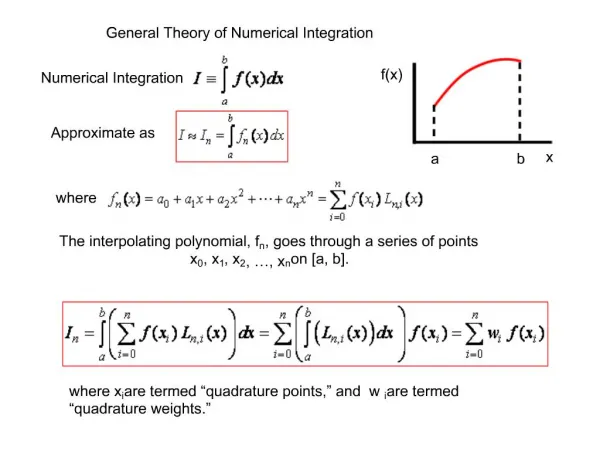
Numerical Integration. CSE245 Lecture Notes. Content. Introduction Linear Multistep Formulae Local Error and The Order of Integration Time Domain Solution of Linear Networks. Transient analysis is to obtain the transient response of the circuits.

E N D
Numerical Integration CSE245 Lecture Notes
Content • Introduction • Linear Multistep Formulae • Local Error and The Order of Integration • Time Domain Solution of Linear Networks
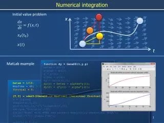
Transient analysis is to obtain the transient response of the circuits. Equations for transient analysis are usually differential equations. Numerical integration: calculate the approximate solutions Xn. Linear multistep formulae are the primary numerical integration method. Introduction
k k iXn-i + h iXn-i = 0 i=0 i=0 Linear Multistep Formulae • Differential equations are X = F(X) • Assume values Xn-1, Xn-2, … , Xn-k and derivatives Xn-1, Xn-2, … , Xn-k are known, the solution Xn and Xn can be approximated by a polynomial of these values:
Linear Multistep Formulae • There are two distinct classes LMS: • Explicit predictors --- 0 = 0 --- Xn is the only unknown variable • Implicit --- 0 0 --- Xn, Xn are all unknown variables.
Linear Multistep Formulae • Three simplest LMS formulae: • The forward Euler • The backward Euler • Trapezoidal
X(t) Xn X(tn) Xn-1 tn tn-1 t Linear Multistep Formulae • The forward Euler Xn– Xn-1– h Xn-1 = 0 where 0 = 1, 1 = -1, 0 = 0, 1 = -1
Linear Multistep Formulae • The backward Euler Xn– Xn-1– h Xn = 0 where 0 = 1, 1 = -1, 0 = -1, 1 = 0 • It is an implicit representation. We may assume some initial value for Xn and iterate to approximate the solution Xn and Xn.
Linear Multistep Formulae • Trapezoidal Xn– Xn-1– h (Xn + Xn-1 )/2= 0 where 0 = 1, 1 = -1, 0 = -1/2, 1 = -1/2 • It is also an implicit representation. Xn, Xn can be obtained through some iterative procedure.
Local Error • Two crucial concepts • Local error --- the error introduced in a single step of the integration routine. • Global error--- the overall error caused by repeated application of the integration formula.
Diverging flow X(t) Converging flow t Global error and local error Local Error
Local Error • Two types of error in each step: • Round-offerror --- due to the finite-precision (floating-point) arithmetic. • Truncationerror --- caused by truncation of the infinite Taylor series, present even with infinite-precision arithmetic.
k k iX(tn-i) + h iX(tn-i) i=1 i=0 Local Error and Order of Integration • Local error Ek for LMS Ek = X(tn) + • Ek can be expanded into Taylor series. If the coefficients of the first pth derivatives are zero, the order of integration is p.
k k i((tn-tn-i)/h)l + h (-l/h)i((tn-tn-i)/h)l-1 i=0 i=0 k i = 0 i=0 k k (ii - i) = 0 [(ii - pi)ip-1] = 0 i=0 i=0 Order of Integration • Let X(t) = ((tn-t)/h)l and tn– tn-i = ih, • Ek = • For pth order integration, the first p+1 elements (l = 0, 1, … , p) will all be zeros: • l = 0 • l = 1 • … • l = p
Order of Integration • The forward Euler 0 = 1, 1 = -1, 0 = 0, 1 = -1 So l = 0 0 + 1 = 1 + (-1) = 0; l = 1 00 + 11 - 0 - 1 = 10 + (-1)1 - 0 – (-1) = 0; l = 2 (11 - 21)1 = ((-1)1 - 2(-1))1 = 1 0; The forward Euler is 1th order.
Order of Integration • The backward Euler 0 = 1, 1 = -1, 0 = -1, 1 = 0 So l = 0 0 + 1 = 1 + (-1) = 0; l = 1 00 + 11 - 0 - 1 = 10 + (-1)1 - (-1) - 0 = 0; l = 2 (11 - 21)1 = ((-1)1 - 20)1 = -1 0; The backward Euler is 1th order.
Order of Integration • Trapezoidal 0 = 1, 1 = -1, 0 = -1/2, 1 = -1/2 So l = 0 0 + 1 = 1 + (-1) = 0; l = 1 00 + 11 - 0 - 1 = 10 + (-1)1 - (-1/2) – (-1/2) = 0; l = 2 (11 - 21)1 = ((-1)1 - 2(-1/2))1 = 0; l = 3 (11 - 31)12 = ((-1)1 - 3(-1/2))1 = 1/2 0; The trapezoidal method is 2th order
Order of Integration • The algorithm for defining and : --- Choose p, the order of the numerical integration method needed; --- Choose k, the number of previous values needed; --- Write down the (p+1) equations of pth order accuracy; --- Choose other (2k-p) constrains of the coefficients and ; --- Combine and solve above (2k+1) equations; --- Get the result coefficients and .
k k iXn-i + h iXn-i = 0 i=0 i=0 Solution of Linear Networks • Combine the differential equations for linear networks and the numerical integration equations: MX = -GX + Pu (1) (2)
k k iXn-i + h iXn-i = 0 i=1 i=1 Solution of Linear Networks (1) Xn + h0Xn + Xn + h0Xn + b = 0 Xn = (-1/h0)( Xn + b) (2)+(3)M[(-1/h0)( Xn + b)] = -GXn + Pu (-1/h0) Xn = -GXn + Pu + (M/h0)b (3)
ic (-C/h0) – (C/h0) bc vc ic vc Solution of Linear Networks • For capacitance C vc = ic C [(-1/h0)( vc + bc)] = ic (-C/h0) vc– (C/h0) bc = ic
il – (L/h0) bl + - vl (-L/h0) il vl Solution of Linear Networks • For inductance L il = vl L [(-1/h0)( il + bl)] = vl (-L/h0) il– (L/h0) bl = vl
References • CK. Cheng, John Lillis, Shen Lin and Norman Chang “Interconnect Analysis and Synthesis”, Wiley and Sons, 2000 • Jiri Vlach and Kishore Singhal “Computer Methods for Circuit Analysis and Design”, 1983