Numerical Integration for Initial Value Problem in MATLAB
This guide discusses initial value problems, numerical integration, and using MATLAB for integration and plotting results of a given system. Learn how to set up, solve, and visualize solutions for DE systems using MATLAB.


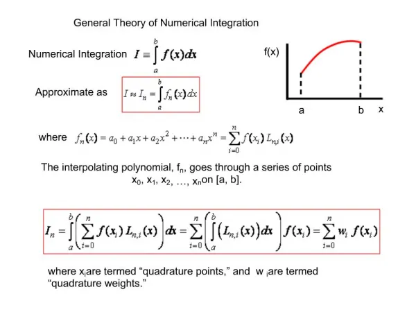
Numerical Integration for Initial Value Problem in MATLAB
E N D
Presentation Transcript
Numerical integration x Initial value problem functiondy = GeneDE(t,y,p) betam = p(1); alpham = p(2); q = p(3); alpha = p(4); dy = zeros(2,1); dy(1) = betam - alpham*y(1); dy(2) = q*y(1) - alpha*y(2); MatLab example betam= 1/10; alpham= 1/30; q = 10; alpha = 1/30;% Parameters MaxTime= 60; % Integration time Yinitial= 0; Yminitial= 0;% Initial conditions [T,Y] = ode45(@GeneDE,[0 MaxTime],[YminitialYinitial],[],[betamalpham q alpha]); h = figure; subplot(2,1,1); plot(T,Y(:,1),'r','LineWidth',2); set(gca,'FontSize',12); title('Model with mRNA and protein explicitly separated: mRNA'); xlabel('t'); ylabel('Ym'); subplot(2,1,2); plot(T,Y(:,2),'LineWidth',2); set(gca,'FontSize',12); title('Model with mRNA and protein explicitly separated: Protein'); xlabel('t'); ylabel('Y'); t
Initial value problem: Equations x Given: How a system state turns into a future system state Given: Initial condition Want: Trajectory of system x0(t0) t
Initial value problem: Illustration x x0(t0) h t
First approximation: Euler method xEULER(t0 + h) x x0(t0) h t
Back up a bit to estimate more representative slope xEULER(t0 + h) x x0(t0) h t
Back up a bit to estimate more representative slope xEULER(t0 + h) x x2ND ORDER(t0 + h) x0(t0) h t
Iterate . . . x x0(t0) t
Iterate again . . . x x0(t0) t
Iterate yet again . . . x x0(t0) t
Error accumulates in the numerical solution x x(t) x0(t0) x2ND ORDER(t) t
Quality control: Adaptive stepsize x x0(t0) h t
Quality control: Adaptive stepsize x x0(t0) h/2 t
Quality control: Adaptive stepsize x x0(t0) t
Quality control: Adaptive stepsize x x0(t0) t
Numerical integration x Initial value problem functiondy = GeneDE(t,y,p) betam = p(1); alpham = p(2); q = p(3); alpha = p(4); dy = zeros(2,1); dy(1) = betam - alpham*y(1); dy(2) = q*y(1) - alpha*y(2); MatLab example betam= 1/10; alpham= 1/30; q = 10; alpha = 1/30;% Parameters MaxTime= 60; % Integration time Yinitial= 0; Yminitial= 0;% Initial conditions [T,Y] = ode45(@GeneDE,[0 MaxTime],[YminitialYinitial],[],[betamalpham q alpha]); h = figure; subplot(2,1,1); plot(T,Y(:,1),'r','LineWidth',2); set(gca,'FontSize',12); title('Model with mRNA and protein explicitly separated: mRNA'); xlabel('t'); ylabel('Ym'); subplot(2,1,2); plot(T,Y(:,2),'LineWidth',2); set(gca,'FontSize',12); title('Model with mRNA and protein explicitly separated: Protein'); xlabel('t'); ylabel('Y'); t
MatLab example x Given: How a system state turns into a future system state Given: Initial condition x0(t0) Want: Trajectory of system t
MatLab example Script: Tell MatLab initial conditions, parameters, and time intervals. functiondy = GeneDE(t,y,p) Integrate the DE system. [T,Y] = ode45(@GeneDE…) Plot results.
Create a file called GeneDE.m Script: Tell MatLab initial conditions, parameters, and time intervals. functiondy = GeneDE(t,y,p) %Extract parameters from p betam= p(1); alpham = p(2); q = p(3); alpha = p(4); % Format output as a column vector dy= zeros(2,1); % Specify differential equations dy(1) = betam - alpham*y(1); dy(2) = q*y(1) - alpha*y(2); Integrate the DE system. [T,Y] = ode45(@GeneDE…) Plot results.
Create a file called RunGeneDE.m Script: Tell MatLab initial conditions, parameters, and time intervals. functiondy = GeneDE(t,y,p) betam = p(1); alpham = p(2); q = p(3); alpha = p(4); dy = zeros(2,1); dy(1) = betam - alpham*y(1); dy(2) = q*y(1) - alpha*y(2); Integrate the DE system. [T,Y] = ode45(@GeneDE…) Plot results.
Fill in RunGeneDE.m and run betam= 1/10; alpham= 1/30; q = 10; alpha = 1/30;% Parameters MaxTime= 60; % Integration time Yinitial= 0; Yminitial= 0;% Initial conditions [T,Y] = ode45(@GeneDE,[0 MaxTime],[YminitialYinitial],[],[betamalpham q alpha]); h = figure; subplot(2,1,1); plot(T,Y(:,1),'r','LineWidth',2); set(gca,'FontSize',12); title('Model with mRNA and protein explicitly separated: mRNA'); xlabel('t'); ylabel('Ym'); subplot(2,1,2); plot(T,Y(:,2),'LineWidth',2); set(gca,'FontSize',12); title('Model with mRNA and protein explicitly separated: Protein'); xlabel('t'); ylabel('Y'); functiondy = GeneDE(t,y,p) betam = p(1); alpham = p(2); q = p(3); alpha = p(4); dy = zeros(2,1); dy(1) = betam - alpham*y(1); dy(2) = q*y(1) - alpha*y(2);