Numerical Integration Methods: Newton-Cotes and Simpson's Rules
Learn about Newton-Cotes Integration, Trapezoidal Rule, Simpson's Rule, error estimation, and applications in numerical analysis.

Numerical Integration Methods: Newton-Cotes and Simpson's Rules
E N D
Presentation Transcript
Numerical Integration Chapter 5 Lecture Notes Mohd Sani Mohamad Hashim Universiti Malaysia Perlis ENT 258 Numerical Analysis
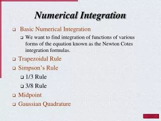
Introduction • Newton-Cotes Integration Formula • Trapezoidal Rule • Simpson’s Rule
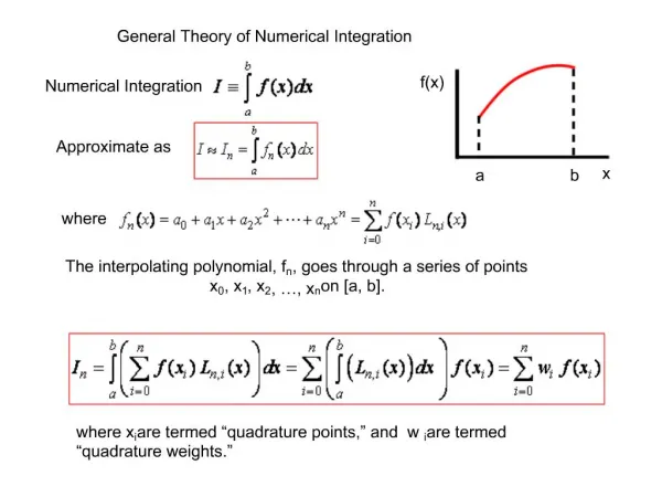
Newton-Cotes Integration • The Newton-Cotes formulas are the most common numerical integration schemes. • They are based on the strategy of replacing a complication or tabulated data with an approximating function
Newton-Cotes Integration A single straight line A single parabola
Newton-Cotes Integration Three straight line segments
Newton-Cotes Integration Closed integration Open integration
The Trapezoidal Rule • The first formula of Newton-Cotes closed integration. • The area under the straight line is • Result of integration is called as the trapezoidal rule
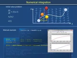
Error of Trapezoidal Rule • An estimation for the local truncation error of a single application of trapezoidal rule is: • (read as xi) lies somewhere in the interval from a to b
Ex. 21.1 • Use trapezoidal rule to numerically integrate: • From a = 0 to b = 0.8. • Exact solution is 1.640533 • Solution: • For f(0) = 0.2 and f(0.8) = 0.232
Solution • Integration by trapezoidal rule: • A percent relative error: (if true value is given)
Solution • Actual situation, approximate error estimate is required. • Average value for second derivative:
Solution • Average value for second derivative:
Solution • Truncation error of trapezoidal rule:
Problem 21.2 • Evaluate the following integral: • (a) Analytically • (b) Single application of trapezoidal rule
Solution • Analytical
Solution • Trapezoidal rule (n = 1): • Trapezoidal rule (n = 2): • Trapezoidal rule (n = 4):
The Multiple-ApplicationTrapezoidal Rule • To improve the accuracy of the trapezoidal rule is to divide the integration interval from a to b into a number of segments and apply the method to each segment. Two segments Three segments
The Multiple-ApplicationTrapezoidal Rule • To improve the accuracy of the trapezoidal rule is to divide the integration interval from a to b into a number of segments and apply the method to each segment. Four segments Five segments
The Multiple-ApplicationTrapezoidal Rule General format for multiple application integrals
The Multiple-ApplicationTrapezoidal Rule • For n segments of equal width: • If a and b are designated as x0 and xn respectively, the total integral is • General form of trapezoidal integration
The Multiple-ApplicationTrapezoidal Rule • The error for multiple-application trapezoidal rule can be obtained by summing the individual errors for each segments • Where: • f”(i) is second derivative at point I located in segment i • It can be simplified by estimating the mean value second derivative:
The Multiple-ApplicationTrapezoidal Rule • It can be simplified by estimating the mean value second derivative: • By assuming , it can be rewritten as truncation error
Ex. 21.2 • Use trapezoidal rule to numerically integrate: • From a = 0 to b = 0.8. • Exact solution is 1.640533 • Solution:
Solution • Three points: • f(0) = 0.2, f(0.4) = 2.456 and f(0.8) = 0.232 • Integration by trapezoidal rule:
Solution • A percent relative error: (if true value is given) • Truncation error:
Problem 21.10 • Evaluate the integration of the following tabular data with the trapezoidal rule:
Solution • Trapezoidal rule (n = 5):
Simpson’s Rule • Simpson’s rule is another way to obtain a more accurate estimate of an integral. Simpson’s 1/3 rule Simpson’s 3/8 rule
Simpson’s 1/3 Rule • By utilizing second-order interpolating polynomial • The integration becomes • After integration and algebraic manipulation • where: h=(b - a)/2
Simpson’s 1/3 Rule • An alternative derivation (Box 21.3) where the Newton-Gregory polynomial is integrated to obtain the same formula. • The Simpson’s 1/3 rule can be express: • where a=x0, b=x2 and x1is the point midway between a & b • Notice that the middle point is weighted by two-thirds and the two end points by one-sixth
Simpson’s 1/3 Rule • Truncation error for single segment application of Simpson’s 1/3 • Because h = (b - a)/2
Ex. 21.4 • Use Simpson’s 1/3 rule to numerically integrate: • From a = 0 to b = 0.8. • Exact solution is 1.640533 • Solution:
Solution • Three points: • f(0) = 0.2, f(0.4) = 2.456 and f(0.8) = 0.232 • Integration by Simpson’s rule:
Solution • A percent relative error: (if true value is given) • Truncation error:
Solution • How to find out f4 () = -2400 ? • Fourth derivative:
Solution • Average value for fourth derivative:
The Multiple-Application Simpson’s 1/3 Rule • For n segments of equal width: • If a and b are designated as x0 and xn respectively, the total integral is • General form of Simpson’s 1/3 rule integration
The Multiple-Application Simpson’s 1/3 Rule • The truncation error of multiple application Simpson’s 1/3 is given as follow
Ex. 21.5 • Use Simpson’s 1/3 rule for multiple-application to numerically integrate: • From a = 0 to b = 0.8. • Exact solution is 1.640533 • Solution:
Solution • Five points: • f(0) = 0.2, f(0.2) = 1.288 • f(0.4) = 2.456, f(0.6) = 3.464 • f(0.8) = 2.232 • Integration by Simpson’s rule:
Solution • A percent relative error: (if true value is given) • Truncation error:
Simpson’s 3/8 Rule • The first formula of a third-order Lagrange polynomial. • where h = (b – a) /3 • This equation is called Simpson’s 3/8 rule
Simpson’s 3/8 Rule • The 3/8 rule can be also be expressed as: • Simpson’s 3/8 truncation error: • Because h = (b – a)/3
The Simpson’s 3/8 Rule 1/3 and 3/8 of Simpson’s rule applied in tandem
Ex. 21.6 • Use Simpson’s 3/8 rule for multiple-application to numerically integrate: • From a = 0 to b = 0.8. • Use it in conjunction with Simpson’s 1/3 rule to integrate the same function • Note: exact solution is 1.640533