NUMERICAL INTEGRATION
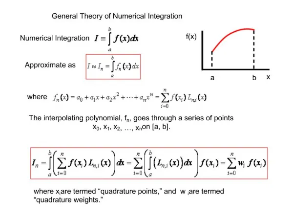
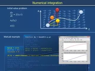
NUMERICAL INTEGRATION. Motivation: Most such integrals cannot be evaluated explicitly. Many others it is often faster to integrate them numerically rather than evaluating them exactly using a complicated antiderivative of f(x) Example:

NUMERICAL INTEGRATION
E N D
Presentation Transcript
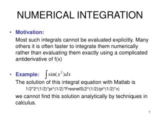
NUMERICAL INTEGRATION • Motivation: Most such integrals cannot be evaluated explicitly. Many others it is often faster to integrate them numerically rather than evaluating them exactly using a complicated antiderivative of f(x) • Example: The solution of this integral equation with Matlab is 1/2*2^(1/2)*pi^(1/2)*FresnelS(2^(1/2)/pi^(1/2)*x) we cannot find this solution analytically by techniques in calculus.
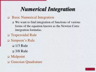
Course content • Methods of Numerical Integration • Trapezoidal Rule’s • 1/3 Simpson’s method • 3/8 Simpson’s method • Applied in two dimensional domain
Trapezoidal Rule’s f fp
Function f approximately by function fp. Then, where fp is a linear polynomial interpolation, that is By substitution u=x-x0we have where
Trapezoidal Rule’s f fp
For two interval, we can use summation operation to derive the formula of two interval trapezoidal that is where
Trapezoidal Rule’s f fp
Similar to two interval trapezoidal, we can derive three interval trapezoidal formula that is where • Thus, for n interval we have where and for
1/3 Simpson’s f fp
Function f approximately by function fp. Then, where fp is a quadratic polynomial interpolation, that is By substitution u=x-x0we have where
1/3 Simpson’s f fp
For 4 subinterval we have where • Thus, for n subinterval we have where and
3/8 Simpson’s fp f
Similar to 1/3 Simpson’s method, f approximately by function fp where fp is a cubic polynomial interpolation, that is By substitution u=x-x0we have where and
Numerical Integration in a Two Dimensional Domain c(x) d(x) b= =a
A double integration in the domain is written as • The numerical integration of above equation is to reduce to a combination of one-dimensional problems
Procedure: • Step 1: Define So, the solution is • Step 2: Divided the range of integration [a,b] into N equispaced intervals with the interval size So, the grid points will be denoted by and then we have
Step 3: Divided the domain of integration into N equispaced intervals with the interval size So, the grid points denoted by • Step 4: By Applying numerical integration for one-dimensional (for example the trapezoidal rule) we have for
Step 5: By applying numerical integration (for example trapezoidal rule) in one-dimensional domain we have the solution of double integration is