
Sparse LU Factorization without Pivoting for Solving Ax=b
E N D
Presentation Transcript
Sparse LU FactorizationWithout Pivoting Note: slides for sparse-sparse triangular solve are at the end of the April 9 slide set.
Symmetric or Nonsymmetric Ax = b: Gaussian elimination without pivoting • Factor A = LU • Solve Ly = b for y • Solve Ux = y for x • Variations: • Pivoting for numerical stability: PA=LU • Cholesky for symmetric positive definite A: A = LLT • Permuting A to make the factors sparser = x
for column j = 1 to n do solve scale:lj = lj / ujj j U L A ( ) L 0L I ( ) ujlj L = aj for uj, lj Left-looking Column LU Factorization • Column j of A becomes column j of L and U
L = speye(n);for column j = 1 : ndfs in G(LT) to predict nonzeros of x; x(1:n) = A(1:n, j); // x is a SPA for i = nonzero indices of x in topological order x(i) = x(i) / L(i, i); x(i+1:n) = x(i+1:n) – L(i+1:n, i) * x(i); U(1:j, j) = x(1:j); L(j+1:n, j) = x(j+1:n);cdiv: L(j+1:n, j) = L(j+1:n, j) / U(j, j); Left-looking sparse LU without pivoting (simple)
for j = 1 : n L(j:n, j) = A(j:n, j); for k < j with L(j, k) nonzero % sparse cmod(j,k) L(j:n, j) = L(j:n, j) – L(j, k) * L(j:n, k); end; % sparse cdiv(j) L(j, j) = sqrt(L(j, j)); L(j+1:n, j) = L(j+1:n, j) / L(j, j); end; j LT L A L Sparse Column Cholesky Factorization • Column j of A becomes column j of L
Sparse Cholesky factorization to solve Ax = b • Preorder: replace A by PAPT and b by Pb • Independent of numerics • Symbolic Factorization: build static data structure • Elimination tree • Nonzero counts • Supernodes • Nonzero structure of L • Numeric Factorization: A = LLT • Static data structure • Supernodes use BLAS3 to reduce memory traffic • Triangular Solves: solve Ly = b, then LTx = y
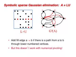
3 7 1 3 7 1 6 8 6 8 4 10 4 10 9 2 9 2 5 5 Predicting the structure of L: Symbolic factorization Fill:new nonzeros in factor Symmetric Gaussian elimination: for j = 1 to n add edges between j’s higher-numbered neighbors G+(A)[chordal] G(A)
Path lemma [Davis Thm 4.1] Let G = G(A) be the graph of a symmetric, positive definite matrix, with vertices 1, 2, …, n, and let G+ = G+(A)be the filled graph. Then (v, w) is an edge of G+if and only if G contains a path from v to w of the form (v, x1, x2, …, xk, w) with xi < min(v, w) for each i. (This includes the possibility k = 0, in which case (v, w) is an edge of G and therefore of G+.)
3 7 1 6 8 10 4 10 9 5 4 8 9 2 2 5 7 3 6 1 Elimination Tree G+(A) T(A) Cholesky factor T(A) : parent(j) = min { i > j : (i, j) inG+(A) } parent(col j) = first nonzero row below diagonal in L • T describes dependencies among columns of factor • Can compute G+(A) easily from T • Can compute T from G(A) in almost linear time
Finding the elimination tree efficiently • Given the graph G = G(A) of n-by-n matrix A • start with an empty forest (no vertices) • for i = 1 : n add vertex i to the forest for each edge (i, j) of G with i > j make i the parent of the root of the tree containing j • Implementation uses a disjoint set union data structure for vertices of subtrees • Running time is O(nnz(A) * inverse Ackermann function) • In practice, we use an O(nnz(A) * log n) implementation
Facts about elimination trees • If G(A) is connected, then T(A) is connected (it’s a tree, not a forest). • If A(i, j) is nonzero and i > j, then i is an ancestor of j in T(A). • If L(i, j) is nonzero, then i is an ancestor of j in T(A). [Davis Thm 4.4] • T(A) is a depth-first spanning tree of G+(A). • T(A) is the transitive reduction of the directed graph G(LT).
Describing the nonzero structure of L in terms of G(A) and T(A) • If (i, k) is an edge of G with i > k, then the edges of G+ include: (i, k) ; (i, p(k)) ; (i, p(p(k))) ; (i, p(p(p(k)))) . . . • Let i > j. Then (i, j) is an edge of G+ iff j is an ancestor in T of some k such that (i, k) is an edge of G. • The nonzeros in row i of L are a “row subtree” of T. • The nonzeros in col j of L are some ofj’s ancestors in T. • Just the ones adjacent in G to vertices in the subtree of T rooted at j.
Symbolic factorization: Computing G+(A) T and G give the nonzero structure of L either by rows or by columns. • Row subtrees[Davis Fig 4.4]: Tr[i] is the subtree of T formed by the union of the tree paths from j to i, for all edges (i, j) of G with j < i. • Tr[i] is rooted at vertex i. • The vertices of Tr[i] are the nonzeros of row i of L. • For j < i, (i, j) is an edge of G+ iff j is a vertex of Tr[i]. • Column unions[Davis Fig 4.10]: Column structures merge up the tree. • struct(L(:, j)) = struct(A(j:n, j)) + union( struct(L(:,k)) | j = parent(k) in T ) • For i > j, (i, j) is an edge of G+ iff either (i, j) is an edge of G or (i, k) is an edge of G+ for some child k of j in T. • Running time is O(nnz(L)), which is best possible . . . • . . . unless we just want the nonzero counts of the rows and columns of L
Finding row and column counts efficiently • First ingredient: number the elimination tree in postorder • Every subtree gets consecutive numbers • Renumbers vertices, but does not change fill or edges of G+ • Second ingredient: fast least-common-ancestor algorithm • lca (u, v) = root of smallest subtree containing both u and v • In a tree with n vertices, can do m arbitrary lca() computationsin time O(m * inverse Ackermann(m, n)) • The fast lca algorithm uses a disjoint-set-union data structure
Row counts • RowCnt(u) is # vertices in row subtree Tr[u]. • Third ingredient: path decomposition of row subtrees • Lemma: Let p1 < p2 < … < pk be some of the vertices of a postordered tree, including all the leaves and the root. Let qi = lca(pi , pi+1) for each i < k. Then each edge of the tree is on the tree path from pj to qj for exactly one j. • Lemma applies if the tree is Tr[u] and p1, p2, …, pk are the nonzero column numbers in row u of A. • RowCnt(u) = 1 + sumi ( level(pi) – level( lca(pi , pi+1) ) • Algorithm computes all lca’s and all levels, then evaluates the sum above for each u. • Total running time is O(nnz(A) * inverse Ackermann)
Column counts • ColCnt(v) is computed recursively from children of v. • Fourth ingredient: weights or “deltas” give difference between v’s ColCnt and sum of children’s ColCnts. • Can compute deltas from least common ancestors. • See Davis section 4.5 (or GNP paper, web site) for details • Total running time is O(nnz(A) * inverse Ackermann)
Sparse Cholesky factorization to solve Ax = b • Preorder: replace A by PAPT and b by Pb • Independent of numerics • Symbolic Factorization: build static data structure • Elimination tree • Nonzero counts • Supernodes • Nonzero structure of L • Numeric Factorization: A = LLT • Static data structure • Supernodes use BLAS3 to reduce memory traffic • Triangular Solves: solve Ly = b, then LTx = y
Complexity measures for sparse Cholesky • Space: • Measured by fill, which is nnz(G+(A)) • Number of off-diagonal nonzeros in Cholesky factor (need to store about n + nnz(G+(A)) real numbers). • Sum over vertices of G+(A) of (# of higher neighbors). • Time: • Measured by number of flops(multiplications, say) • Sum over vertices of G+(A) of (# of higher neighbors)2 • Front size: • Related to the amount of “fast memory” required • Max over vertices of G+(A) of (# of higher neighbors).
3 7 1 6 8 4 10 9 2 5 Complexity measures for chordal completion Elimination degree: dj = # higher neighbors of j in G+ d = (2, 2, 2, 2, 2, 2, 1, 2, 1, 0) G+(A) Nonzeros = edges = Σjdj(moment 1) Work = flops = Σj(dj)2(moment 2) Front size = treewidth = maxjdj(moment ∞) Treewidth shows up in lots of other graph algorithms…
n1/2 n1/3 Complexity of direct methods Time and space to solve any problem on any well-shaped finite element mesh