Understanding Basic Statistical Concepts and the Least-Squares Method

1. Basic statistical concepts and least-squares. Sat05_61.ppt, 2005-11-28. • Statistical concepts • Distributions • Normal-distribution 2. Linearizing 3. Least-squares • The overdetermined problem • The underdetermined problem

2. Histogram. Describes distribution of repeated observations At different times or places ! Distribution of global 10 mean gravity anomalies

3. Statistic: Distributions describes not only random events ! We use statistiscal description for ”deterministic” quantities as well as on random quantities. Deterministic quantities may look as if they have a normal distribution !

4. ”Event” Basic concept: Measured distance, temperature, gravity, … Mapping: Stocastisc variabel . In mathematics: functional, H – function-space – maybe Hilbertspace. Gravity acceleration in point P: mapping of the space of all possible gravity-potentials to the real axis.

5. Probability-density , f(x): What is the probability P that the value is in a specific interval:

6. Mean and variance, Estimation-operator E:

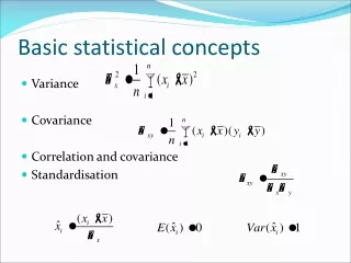
7. Variance-covariance in space of several dimensions: Mean value and variances:

8. Correlation and covariance-propagation: Correlation between two quantities: = 0: independent. Due to linearity

9. Mean-value and variance of vector If X and A0 are vectors of dimension n and A is an n x m matrix, then The inverse P = generally denoted the weight-matrix

10. Distribution of the sum of 2 numbers: • Exampel Here n = 2 and m = 1. We regard the sum of 2 observations: • What is the variance, if we regard the difference between two observations ?

11. Normal-distribution 1-dimensional quantity has a normal distribution if • Vektor of simultaneously normal-distributed quantities if • n-dimensional normal distribution.

12. Covarians-propagation in several dimensions: X: n-dimensional, normally distributed, D nxm matrix , then Z=DZ also normal distributed, E(Z)=D E(X)

13. Estimate of mean, variance etc

14. Covarians function If the covariance COV(x,y) is a function of x,y then we have a Covarians-function May be a function of • Time-difference (stationary) • Spherical Distance, ψ on the unit-sphere (isotrope)

15. Normally distributed data and resultat. If data are normaly dsitributed, then the resultats are also normaly distributed If they are linearily related ! We must linearize – TAYLOR-Development with only 0 and 1. order terms. Advantage: we may interprete error-distributions.

16. Distributions in infinite-dimensional spaces V( P) element in separable Hilbert-space: Normal distributed with sum of variances finite !

17. Stochastic process. What is the probability P for the event is located in a specific interval Exampel: What is the probability that gravity in Buddinge lies in between -20 and 20 mgal and that gravity in Rockefeller lies in the same interval

18. Stokastisc process in Hilbertspace What is the mean value and variance of ”the Evaluation-functional”,

19. Covariance function of stationary time-series. Covariance-function depends only on |x-y| Variances called ”Power-spectrum”.

20. Covariance function – gravity-potential. • Suppose Xij normal-distributed with the same variance for constant ”i”.

21. Isotropic Covariance-function for Gravity potential

22. Linearizering: why ? We want to find best estimate (X) for m quantities from n observations (L). Data normal-distributed, implies result normaly distributed, if there is a linear relationship. If m > n there exist an optimal metode for estimating X: Metode of Least-Squares

23. Linearizing – Taylor-development. If non-linear: Start-værdi (skøn) for X kaldes X1 Taylor-development with 0 og 1. order terms after changing the order

24. Covariance-matrix for linearizered quantities If measurements independently normal distributed with varians-covariance Then the resultatet y normal-dsitributed with variance-covarians:

25. Linearizing the distance-equation. Linearized based on coordinates

26. On Matrix form: If 3 equations with 3 un-knowns !

27. Numerical-example If (X11, X12,X13) = ( 3496719 m, 743242 m, 5264456 m). Satellite: (19882818.3, -4007732.6 , 17137390.1) Computed distance: 20785633.8 m Measured distance: 20785631.1 m ((3496719.0-19882818.3)dX1 + (743242.0-4007732.6) dX2+(5264456 .0-17137390.1) dX3)/20785633.8 = ( 20785631.1 - 20785633.8) or: -0.7883 dX1 -0.1571 dX2 + 1.7083 dX3 = -2.7

28. Linearizing in Physical Geodesy based on T=W-U In function-spaces the Normal-potential may be regarded as a 0-order term in a Taylor-development.We may differentiate in Metric space (Frechet-derivative).

29. Method of Least-Square. Over-determined problem. More observations than parameters or quantities which must be estimated: Examples: GPS-observations, where we stay at the same place (static) We want coordinates of one or more points. Now we suppose that the unknowns are m linearily independent quantities !

30. Least-squares = Adjustment. • Observation-equations: • We want a solution so that Differentiation:

31. Metod of Last-Squares. Variance-covariance.

32. Metod of Least-Squares. Linear problem. Gravity observations: H, g=981600.15 +/-0.02 mgal 12.11+/-0.03 -22.7+/-0.03 G 10.52+/-0.03 I

33. Observations-equations..

34. Method of Least-Squares. Over-determined problem. Compute the varianc-covariance-matrix

35. Method of Least-Squares. Optimal if observations are normaly distributed + Linear relationship ! Works anyway if they are not normally distributed ! And the linear relationship may be improved using iteration. Last resultat used as a new Taylor-point. Exampel: A GPS receiver at start.

36. Metode of Least-Squares. Under-determined problem. We have fewer observations than parameters: gravity-field, magnetic field, global temperature or pressure distribution. We chose a finite dimensional sub-space, dimension equal to or smaller than number of observations. Two possibilities (may be combined): • We want ”smoothest solution” = minimum norm • We want solution, which agree as best as possible with data, considering the noise in the data

37. Method of Least-Squares. Under-determined problem. Initially we look for finite-dimensional space so the solution in a variable point Pi becomes a linear-combination of the observations yj: If stocastisk process, we want the ”interpolation-error” minimalized

38. Method of Least-Squares. Under-determined problem. Covariances: Using differentiation: Error-variance:

39. Method of Least-Squares. Gravity-prediction. R 4 km 8 km Example: Covarianses: COV(0 km)= 100 mgal2 COV(10 km)= 60 mgal2 COV(8 km)= 80 mgal2 COV(4 km)= 90 mgal2 Q 10 mgal P 6 mgal 10 km

40. Method of Least-Squares. Gravity prediction. Continued: Compute the error-estimate for the anomaly in R.

41. Least-Squares Collocation. Also called: optimal linear estimation For gravity field: name has origin from solution of differential-equations, where initial values are maintained. Functional-analytic version by Krarup (1969) Kriging, where variogram is used closely connected to collocation.

42. Least-Squares collocation. We need covariances – but we only have one Earth. Rotate Earth around gravity centre and we get (conceptually) a new Earth. Covariance-function supposed only to be dependent on spherical distance and distance from centre. For each distance-interval one finds pair of points, of which the product of the associated observations is formed and accumulated. The covariance is the mean value of the product-sum.

43. Covarians-function for gravity anomalies, r=R.

44. Covarians function for gravity-anomalies: Different models for degree-variances (Power-spectrum): Kaula, 1959, (but gravity get infinite variance) Tscherning & Rapp, 1974 (variance finite).