Download
1 / 3
30 likes | 77 Vues
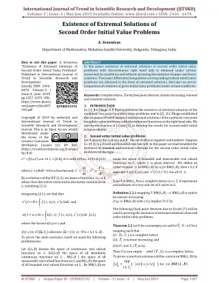
In this paper existence of extremal solutions of second order initial value problems with discontinuous right hand side is obtained under certain monotonicity conditions and without assuming the existence of upper and lower solutions. Two basic differential inequalities corresponding to these initial value problems are obtained in the form of extremal solutions. And also we prove uniqueness of solutions of given initial value problems under certain conditions. A. Sreenivas "Existence of Extremal Solutions of Second Order Initial Value Problems" Published in International Journal of Trend in Scientific Research and Development (ijtsrd), ISSN: 2456-6470, Volume-3 | Issue-4 , June 2019, URL: https://www.ijtsrd.com/papers/ijtsrd25192.pdf Paper URL: https://www.ijtsrd.com/mathemetics/other/25192/existence-of-extremal-solutions-of-second-order-initial-value-problems/a-sreenivas<br>

E N D
International Journal of Trend in Scientific Research and Development (IJTSRD) Volume: 3 | Issue: 4 | May-Jun 2019 Available Online: www.ijtsrd.com e-ISSN: 2456 - 6470 Existence of Extremal Solutions of Second Order Initial Value Problems A. Sreenivas Department of Mathematics, Mahatma Gandhi University, Nalgonda, Telangana, India How to cite this paper: A. Sreenivas "Existence of Extremal Solutions of Second Order Initial Value Problems" Published in International Journal of Trend in Scientific Research and Development (ijtsrd), ISSN: 2456- 6470, Volume-3 | Issue-4, June 2019, pp.1657-1659, URL: https://www.ijtsrd.c om/papers/ijtsrd25 192.pdf Copyright © 2019 by author(s) and International Journal of Trend in Scientific Research and Development Journal. This is an Open Access article distributed under the terms of the Creative Commons Attribution License (CC BY 4.0) (http://creativecommons.org/licenses/ by/4.0) x11 = f(t,x,x1)a.a. t∈I1 = [0,A], A>o with x(0)=a, x1(0)=b (2.1) ABSTRACT In this paper existence of extremal solutions of second order initial value problems with discontinuous right hand side is obtained under certain monotonicity conditions and without assuming the existence of upper and lower solutions. Two basic differential inequalities corresponding to these initial value problems are obtained in the form of extremal solutions. And also we prove uniqueness of solutions of given initial value problems under certain conditions. Keywords: Complete lattice, Tarski fixed point theorem, isotone increasing, minimal and maximal solutions. 1.INTRODUCTION In [1], B C Dhage ,G P Patil established the existence of extremal solutions of the nonlinear two point boundary value problems and in [2] , B C Dhage established the existence of weak maximal and minimal solutions of the nonlinear two point boundary value problems with discontinuous functions on the right hand side. We use the mechanism of [1]and [2] ,to develop the results for second order initial value problems. 2.Second order initial value problems Let R denote the real line and R+ , the set of all non negative real numbers. Suppose I1= [0, A] is a closed and bounded interval in R. In this paper we shall establish the existence of maximal and minimal solutions for the second order initial value problems of the type mean the space of bounded and measurable real valued functions on I1, where I1 is given interval . We define an order relation ≤ in BM(I1,R) by x,y∈BM(I1,R), then x≤y if and only if x(t)≤y(t) and A set S in BM(I1, R) is a complete lattice w.r.t ≤ if supremum and infimum of every sub set of S exists in S. Definition 2.1 Amapping T: BM(I1,R) → BM(I1,R) is said to be isotone increasing if x,y∈BM(I1,R) with x≤y implies Tx≤Ty. The following fixed point theorem due to Tarski [7] will be used in proving the existence of extremal solutions of second order initial value problems. Theorem2.2 Let E be a nonempty set and let mapping such that (i)(E, ≤ ) is a complete lattice (ii) (iii)F= {u∈E / Then F is non empty To prove a result on existence define a norm on BM(I1, R) by ( 1 1 t I ∈ IJTSRD25192 2 dx dt d x dt = = where f : I1xRxR→R is a function and 1 11 , x x . for all t∈ I1. ≤ 1 1 ( ) ( ) x t y t 2 By a solution x of the IVP (2.1), we mean a function x : I1→R whose first derivative exists and is absolutely continuous on I1,satisfying (2.1). Integrating (2.1), we find that t x t b f s x s x s ds = +∫ 1 1 ( ) ( , ( ), ( )) and 0 t +∫ = a bt + 1 ( ) x t ( , ) k t s f s x s x s ( , ( ), ( )) ds (2.2) 0 where the kernel k(t,s)=t-s and ( , ) ( , ) k t s C ∈ Ω To prove the main existence result we need the following preliminaries. Let C(I1,R) denote the space of continuous real valued functions on I1, AC(I1,R) the space of all absolutely continuous functions on I1 , M(I1,R ) the space of all measurable real valued functions on I1 and B(I1,R), the space of all bounded real valued functions on I1 . By BM(I1,R),we 1T : E→E be a Ω = ≤ ≤ ≤ {( , ):0 t s } I wherein s t A . 1 1T is isotone increasing and 1T u=u}. and F ≤ is a complete lattice. ( , ) sup ) ∈ = + 1 ( , ) ( ) x t ( ) x BM I R x x t for . 1 @ IJTSRD | Unique Paper ID – IJTSRD25192 | Volume – 3 | Issue – 4 | May-Jun 2019 Page: 1657
International Journal of Trend in Scientific Research and Development (IJTSRD) @ www.ijtsrd.com eISSN: 2456-6470 Then clearly BM(I1,R) is a Banach space with the above norm. We shall now prove the existence of maximal and minimal solutions for the IVP (2.1). For this we need the following assumptions: (f1): f is bounded on I1xRxR by k3 , k3 >0. (f2) : f (t,ϕ (t),ϕ1(t) ) is Lebesgue measurable for Lebesgue measurable functions ϕ ,ϕ1 on I1, and (f3) : f (t,x,x1) is nondecreasing inboth x and x1 in R for a.a. t∈I1. Theorem 2.3 Assume that the hypotheses (f1-f3) hold. Then the IVP (2.1) has maximal and minimal solutions on I1. Proof . Define a sub set S of the Banach space BM(I1,R) by { ( , ): S x BM I R x = ∈ ≤ t ∫ a bt = + + t s − 1 ( ) ( ) ( , ( ), ( )) f s x s x s ds T x t 0 t ∫ a bt ≤ + + ) ( , ( ), ( )) t s f s y s y s ds T y t − = ∀ ∈ 1 ( ( ) t I 1 0 and t ∫ = + 1 1 ( ) ( , ( ), ( )) f s x s x s ds T x t b 0 t ∫ ≤ + = ∈ 1 1 ( , ( ), ( )) f s y s y s ds T y t ( ) , . b t I 1 0 This shows that T is isotone increasing on S. In view of Theorem 2.2, it follows that the operator equation Tx= xhas solutions and that the set of all solutions is a complete lattice, implying that the set of all solutions of (2.1) is a complete lattice. Consequently the IVP (2.1) has maximal and minimal solutions in S. Finally in view of the definition of the operator T,it follows that these extremal solutions are in C(I1,R)⊂AC(I1,R). This completes the proof. We shall now show that the maximal and minimal solutions of the IVP (2.1) serve as the bounds for the solutions of the differential inequalities related to the IVP (2.1). Theorem 2.4 Assume that all the conditions of Theorem 2.3 are satisfied. Suppose that there exists a function u∈S, where S is as defined in the proof of Theorem 2.3 satisfying ( , , ) u f t u u ≤ Then there exists a maximal solution such that 1 ( ) ( ), M u t x t t I ≤ ∈ . Proof. Let p = Sup S. Clearly the element p exists, since S is a complete lattice. Consider the lattice interval [u, p] in S where u is a solution of (2.5) .We notice that [u, p] is obviously a complete lattice. It can be shown as in the proof of Theorem 2.3 that T : [u, p] → S is isotone increasing on [u,p] . We show that T maps [u, p] into itself. For this it suffices to show that u≤Tx for any x∈ S with u≤x. Now from the inequality (2.5), it follows that t u t b f s u s u s ds ≤ +∫ *} k (2.3) 1 3 1 2 A + + + + ( , ) a b A k b k A k where k3* =Max . 3 3 3 2 Clearly S is closed, convex and bounded sub set of the Banach space BM(I1,R) and hence by definition (S,≤) is a complete lattice. We define an operator T : S→BM(I1,R) by t T x t a bt t s f s x s x s = + + − ∫ , t∈I1. (2.4) 1 ( ) ( ) ( , ( ), ( )) ds 0 Then t = +∫ , t∈I1 1 1 ( ) ( , ( ), f s x s x s ds ( )) x t b T 0 Obviously (Tx) and (Tx1) are continuous on I1 and hence measurable on I1 . We now show that T maps S into itself .Let x∈Sbe an arbitrary point , then t T x t a b t t s ≤ + + − ∫ a.a. t∈ I1 with u(0 ) = a , = 11 1 1(0) u b . (2.5) x 1 of the IVP (2.1) ( ) ( ) ( , ( ), f s x s x s ( )) ds M 0 2 t ≤ + + a b t k 3 2 And t +∫ ≤ 1 1 ( ) ( , ( ), f s x s x s ( )) T x t b ds 0 ≤ + b k t 3 Therefore sup t ∈ ( ) = + 1 ( ) ( ) T x T x t T x t I 1 1 1 1 ( ) ( , ( ), ( )) 0 sup t ∈ 2 t t ≤ + + + + a b t k b k t ∫ ≤ + = ∈ 1 1 ( , ( ), f s x s x s ds ( )) ( ) , b T x t t I 3 3 And I 2 1 1 0 t ∫ ≤ a bt + + − 1 ( ) ( ) ( , ( ), s f s u s u s ( )) u t t ds 2 A ≤ + + + + ≤ * a b A k b k A k 0 3 3 3 2 = Tx(t) for all t∈ I1. t ∫ ≤ a bt + + − 1 ( ) ( , ( ), s f s x s x s ds ( )) t 0 This shows that Tmaps S into itself. Let x, y be such that x≤y, then by (f3) we get This shows that Tmaps [u, p] into itself. Applying the Theorem 2.2, we conclude that there is a maximal @ IJTSRD | Unique Paper ID – IJTSRD25192 | Volume – 3 | Issue – 4 | May-Jun 2019 Page: 1658
International Journal of Trend in Scientific Research and Development (IJTSRD) @ www.ijtsrd.com eISSN: 2456-6470 That is sup t I ∈ x solution of the IVP (2.1) in [u, p]. Therefore ( ) ( t x t u M ≤ This completes the proof. Theorem 2.5 Suppose that all the conditions of Theorem 2.3 hold, and assume that there is a function v∈S, where S is as defined in the proof of Theorem 2.3, such that 11 1 ( , , ) v f t v v ≥ Then there is a minimal solution xm of the IVP (2.1) such that xm(t) ≤ v(t) , for t∈I1 . The proof is similar to that of Theorem 2.4 and we omit the details We shall now prove the uniqueness of solutions of the IVP (2.1). Theorem 2.6 In addition to the hypothesis of Theorem 2.3, if the function ( , , ) f t x x on I1 x R x R satisfies the condition that of the integral equation (2.2) and consequently M t ( ) ∫ − ≤ − − Ls ( ) ( t )( ) t ( ) T x T x M x x t s e ds 3 M m M m 2 1 0 Lt e L for t∈I1. ) ≤ − M x x . M m 2 2 This implies that M L − ≤ − T x T x x x . M m M m 2 2 2 a.a. t ∈I1 with v (0 ) = a , = 1(0) v b . M L < , the mapping T is a contrition .Applying the 1 Since 2 contraction mapping principle, we conclude that there exists a unique fixed point x∈ BM(I1,R) such that (Tx)(t) = t x t a bt t s f s x s x s ds = + + − ∫ ∀ ∈ 1 ( ) ( ) ( , ( ), ( )) t I . 1 0 This completes the proof. Acknowledgements: I am thankful to Pro.K.Narsimhareddy for his able guidance. Also thankful to Professor Khaja Althaf Hussain Vice Chancellor of Mahatma Gandhi University, Nalgonda to provide facilities in the tenure of which this paper was prepared. References [1]B.C. Dhage and G.P. Patil “ On differential inequalities for discontinuous non-linear two point boundary value problems” Differential equations and dynamical systems, volume 6, Number 4, October 1998, pp. 405 – 412. 1 − 1 1 x + y − − x y A x y A x + − (2.6) − ≤ 1 1 ( , , ) f t x x ( , , ) f t y y , M Min 1 1 y for some M>0. Then the IVP (2.1) has unique solution defined on I1. Proof . Let BM(I1, R) denote the space of all bounded and measurable functions defined on I1 .Define a norm on BM(I1, R) by sup ( ) x e x t t I ∈ − = , for x∈ BM (I1, R) Lt [2]B.C.Dhage , “On weak Differential Inequalities for nonlinear discontinuous boundary value problems and Applications’’. Differential equations and dynamical systems, volume 7, number 1, January 1999, pp.39-47. 2 1 M L < .Notice 1 where L is a fixed positive constant such that 2 2. . Define T: that BM(I1, R) is a Banach space with the norm BM(I1,R) → BM(I1,R) by (2.4). Let ( ), ( ) m M x t x t be minimal and maximal solutions of the IVP (2.1 ) respectively. Then we have (T M x )(t) - (T t t s f s x s x s − ∫ [3]K. Narshmha Reddy and A.Sreenivas “On Integral Inequities in n – Independent Variables”, Bull .Cal .Math. Soc ., 101 (1) (2009), 63-70 . [4]G. Birkhoff , “Lattice theory ’’ , Amer .Math. Soc. Coll.publ. Vol.25, NewYork, 1979. [5]S.G. Deo, V.Lakshmikantham, V.Raghavendra, “Text book of Ordinary Differential Equations” second edition. m x )(t) = − 1 1 ( ) ( , ( ), ( )) ( , ( ), s x ( )) s f s x ds . M M m m [6]B.C.Dhage “ Existence theory for nonlinear functional boundary value Problems’’. Electronic Journal of Qualitative theory of Differential Equations, 2004, No 1, 1-15. 0 Using (2.6) we see that − x + ( )( ) ( t )( ) t T x T x M m [7]A. Tarski , “A lattice theoretical fixed point theorem and its application, pacific . J. Math., 5(1955), 285 – 310. − t ( ) s x ( ) x s x s − ∫ ≤ − M m ( ) M t s ds ( ) s ( ) A M m 0 @ IJTSRD | Unique Paper ID – IJTSRD25192 | Volume – 3 | Issue – 4 | May-Jun 2019 Page: 1659