Preprocessing of Low Response Data for Predictive Modeling
40 likes | 55 Vues
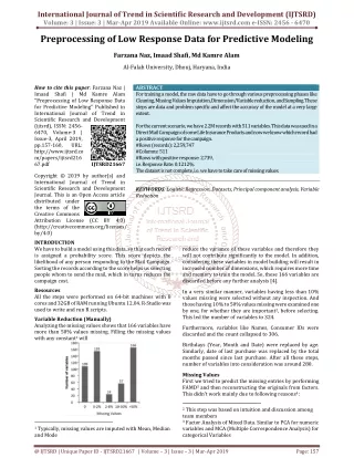
For training a model, the raw data have to go through various preprocessing phases like Cleaning, Missing Values Imputation, Dimension Variable reduction, and Sampling. These steps are data and problem specific and affect the accuracy of the model at a very large extent. For the current scenario, we have 2.2M records with 511 variables. This data was used in a Direct Mail Campaign of some Life Insurance Products and now we know which record had a positive response for the campaign. Rows records 2,259,747 Columns 511 Rows with positive response 2,739, i.e. Response Rate 0.1212 . The dataset is not complete, i.e. we have to take care of missing values. Farzana Naz | Imaad Shafi | Md Kamre Alam "Preprocessing of Low Response Data for Predictive Modeling" Published in International Journal of Trend in Scientific Research and Development (ijtsrd), ISSN: 2456-6470, Volume-3 | Issue-3 , April 2019, URL: https://www.ijtsrd.com/papers/ijtsrd21667.pdf Paper URL: https://www.ijtsrd.com/engineering/computer-engineering/21667/preprocessing-of-low-response-data-for-predictive-modeling/farzana-naz<br>

Preprocessing of Low Response Data for Predictive Modeling
E N D
Presentation Transcript
International Journal of Trend in Scientific Research and Development (IJTSRD) Volume: 3 | Issue: 3 | Mar-Apr 2019 Available Online: www.ijtsrd.com e-ISSN: 2456 - 6470 Preprocessing of Low Response Data for Predictive Modeling Farzana Naz, Imaad Shafi, Md Kamre Alam Al-Falah University, Dhouj, Haryana, India ABSTRACT For training a model, the raw data have to go through various preprocessing phases like Cleaning, Missing Values Imputation, Dimension/Variable reduction, and Sampling. These steps are data and problem specific and affect the accuracy of the model at a very large extent. For the current scenario, we have 2.2M records with 511 variables. This data was used in a Direct Mail Campaign of some Life Insurance Products and now we know which record had a positive response for the campaign. #Rows (records): 2,259,747 #Columns: 511 #Rows with positive response: 2,739, i.e. Response Rate: 0.1212%. The dataset is not complete, i.e. we have to take care of missing values. KEYWORDS:Logistic Regression, Datasets, Principal component analysis, Variable Reduction How to cite this paper: Farzana Naz | Imaad Shafi | Md Kamre Alam "Preprocessing of Low Response Data for Predictive Modeling" Published in International Journal of Trend in Scientific Research and Development (ijtsrd), ISSN: 2456- 6470, Volume-3 | Issue-3, April 2019, pp.157-160, URL: http://www.ijtsrd.co m/papers/ijtsrd216 67.pdf Copyright © 2019 by author(s) and International Journal of Trend in Scientific Research and Development Journal. This is an Open Access article distributed under the terms of the Creative Commons Attribution License (CC BY 4.0) (http://creativecommons.org/licenses/ by/4.0) INTRODUCTION We have to build a model using this data, so that each record is assigned a probability score. This score depicts the likelihood of any person responding to the Mail Campaign. Sorting the records according to the score helps us selecting people whom to send the mail, which in turns reduces the campaign cost. Resources All the steps were performed on 64-bit machines with 8 cores and 32GB of RAM running Ubuntu 12.04. R-Studio was used to write and run R scripts. Variable Reduction (Manually) Analyzing the missing values shows that 166 variables have more than 50% values missing. Filling the missing values with any constant1 will IJTSRD21667 reduce the variance of these variables and therefore they will not contribute significantly to the model. In addition, considering these variables in model building will result in increased number of dimensions, which requires more time and memory to train the model. So, these 166 variables are discarded before any further analysis [4]. In a very similar manner, variables having less than 10% values missing were selected without any inspection. And those having 10% to 50% values missing were examined one by one, for whether they are important2, before selecting. This led the number of variables to 324. Furthermore, variables like Names, Consumer IDs were discarded and the count collapsed to 306. Birthdays (Year, Month and Date) were replaced by age. Similarly, date of last purchase was replaced by the total months passed since last purchase. After all these steps, number of variables into consideration was around 280. Missing Values First we tried to predict the missing entries by performing FAMD3 and then reconstructing the originals from factors. This didn’t work mainly due to following reasons4: 2 This step was based on intuition and discussion among team members 3 Factor Analysis of Mixed Data. Similar to PCA for numeric variables and MCA (Multiple Correspondence Analysis) for categorical Variables 1 Typically, missing values are imputed with Mean, Median and Mode @ IJTSRD | Unique Paper ID - IJTSRD21667 | Volume – 3 | Issue – 3 | Mar-Apr 2019 Page: 157
International Journal of Trend in Scientific Research and Development (IJTSRD) @ www.ijtsrd.com eISSN: 2456-6470 A.FAMD creates dummy variables for each unique value of categorical variable, demanding more memory than the provided 32GB. B.To solve the memory problem, small sample was tried. But now the problem was with the small number of records corresponding to some categories of the categorical variable. A small selected sample was not able to include all categories, leading to constant value(0)in some columns (dummy) making it impossible to perform FAMD. To avoid the problem, missing values of a column were imputed with median of the available values in that column. Missing values in columns having either 1 or NA (missing) were imputed with 0. Mean could have been used instead of median but we selected the later one due to two reasons: A.Mean of a Boolean variable column will be a real number B.For continuous variables like household area, there were outliers which were distorting the natural position of mean. Anyways, imputing median too will compromise the results compared to if we had used any technique based on PCA, FAMD or other predictive methods[3]. Categorical Variables In the following figure, we can see that initially there are 108 factorvariables; but some of them were discarded during manual variable. reduction step. Of the remaining, those having 2 categories/levels were simply converted to Boolean using dummy variables for each category. For remaining, which have more than 2 categories, following steps were taken: A.Create dummies for each category to convert the variable into Boolean. This expansion of 56 such categorical variables resulted in an indicator matrix of 906 dummy columns. B.Now the aim was to perform PCA on this indicator matrix, but that couldn’t be done on whole 2.2M records due to resource constraints. To resolve the issue, the PCA was performed on randomly selected 400K records, and C.Remaining records were multiplied with the rotation matrix for 15PCs to compute/predict5 the components This way we got new data set with 266 columns containing 58 dummy columns corresponding to 29 categorical (with two levels) variables, 15PCs and 222 original numeric columns. ZIP codes were excluded from the PC computation part, as it had too many levels. A simple idea6 is to replace the ZIP with Longitude and Latitude.[7] Note: n-1 dummy columns are sufficient to represent any categorical variables having n levels. So, instead of 58 dummy columns, 29 could have sufficed[6]. At this stage, we have preprocessed and clean data having 2.2M rows and 266 columns. Preparation of Datasets First of all, the preprocessed data was divided into two parts randomly. First part (70%) for preparing training datasets using various sampling methods, and the rest 30% left untouched for testing purpose. Let us call the first part DS_TRAIN and the second one DS_TEST. Both DS_TRAIN and DS_TEST were sampled randomly and maintain the response rate (≈0.12%) similar to that in the original raw data. A model trained with such a low response data will fail to predict the responded rows. To understand the situation, let us suppose that we have a dataset of 10,000 records. This dataset will contain only 12 positive responses. To maintain the accuracy, model will learn to predict the negative responses and even if it predicts all 10,000 rows as not responded, its accuracy is (10000 10000 (If we replicate the responded rows to increase the data, this problem can be avoided. But the model will be more optimistic,i.e. false positive predictions will increase. But when it comes to assign a score to records rather than to classify them as responded/not-responded, it does good. top 15 components were selected on the basis of variance chart −12 )×100 = 99.88% Figure 3: Variances of top 30 Principal Components over 400K records 4 Can be solved on a machine with little more memory using PCA 5 Levels of a factor variable is the number of categories for that variable 6 Factor class is a data type used in R to store categorical variables. @ IJTSRD | Unique Paper ID - IJTSRD21667 | Volume – 3 | Issue – 3 | Mar-Apr 2019 Page: 158
International Journal of Trend in Scientific Research and Development (IJTSRD) @ www.ijtsrd.com eISSN: 2456-6470 To increase the response rate in training dataset, two different strategies were taken: 1.Three training datasets were prepared using stratified sampling. Records with positive response in DS_TRAIN were replicated via Simple Random Sampling with Replacement to make the response rate to 10%, 15% and 20%. Let us call these sets as DS_TRAIN1A, DS_TRAIN1B and DS_TRAIN1C. 2.DS_TRAIN was divided in two parts: DS_TRAIN_R having all records with response 1, and rest in DS_TRAIN_N. Now DS_TRAIN_N was divided randomly in 10 equal data sets. Then DS_TRAIN_R was appended to each of these sets. So all 10 sets have same responded records but mutually exclusive and exhaustive not-responded records. There is a discussion in machine-learning community about what should be the response rate in the stratified sample. According to some blogs, keeping the ratio to 50% is supposed to be a good strategy. Here, we tried three training sa7mples with 10%, 15% and 20% response rates, and our results shows that there is no need to increase it further. Variable Reduction (Automated) Before training the model, variables were selected for all training datasets using stepwise regression methods: Forward Selection and Backward Elimination[2]. Forward Selection involves starting with no variables in the model, adds variables one by one and compares the statistic9. Similarly, Backward Elimination involves starting with all variables and then testing the model after deletion of variables one by one. We used the method regsubsets from R package leaps forcing in all 15PCs.Getting idea from R-Squared plot, 165 variables were selected from forward method and same number from backward. Intersection of these two sets resulted in 144-155 variables for different datasets Model selection based on R-Squared statistic was consistent with Mallows’s Cp and Residual Sum of Squares. Training and Testing the Models We used Logistic Regression to train the models. For the datasets prepared using first strategy, three models were trained and then were tested on the untouched test dataset, which is 30% of the whole data[1]. Due to very low response in the original data, the model can’t be judged just by observing the confusion matrix. Instead, following method was followed: A.The dataset was sorted in decreasing order of probabilities predicted by the model. B.Then it was divided in 10 equal groups, each called a Decile. C.Number of positive responses in each decile was calculated and its cumulative sum was plotted against deciles. 10% Responses 15%Responses Responses 23.54399 23.66791 39.15737 39.03346 49.19455 51.1772 59.72739 59.35564 67.28625 68.02974 75.5886 75.21685 83.02354 82.89963 88.59975 88.9715 95.66295 95.41512 100 The table shows the percentage of responses captured for all the three training data-sets created using the first strategy. 24.16357 39.4052 49.81413 58.2404 66.41884 75.5886 81.9083 88.35192 95.41512 100 100 Figure 5: Decile Plot for Training Dataset having 15% Responses For the 10 training data sets prepared using 2nd method, average of predicted probabilities by all 10 models was taken as the final score. The results were very similar to what we have here using the first strategy.Note: Models using GBM (Gradient Boosting Machines) and Random forest were also triedon the same datasets by some other team members . They too came up with similar Figure 4: R-Squared and Mallows’s C Plot for Forward Selection 79 We have considered R-Squared, but F-tests, Akaike Information Criterion, Mallows’s Cp etc are also possible @ IJTSRD | Unique Paper ID - IJTSRD21667 | Volume – 3 | Issue – 3 | Mar-Apr 2019 Page: 159
International Journal of Trend in Scientific Research and Development (IJTSRD) @ www.ijtsrd.com eISSN: 2456-6470 Summary and Further Scopes Observing the similarity in results of different models tried, it can be interpreted that results are largely dependent on initial variable selection and sampling strategy followed. Regsubsets showed that there were multiple linear dependencies among variables. These dependencies could be removed by doing a little deep analysis. Also creating n-1 dummy columns for a factor variable with n levels might improve the Principal Components. Relative importance of variables as depicted by the GLM11 shows that more (than 15) principal components can be included. As discussed above, ZIP codes should be replaced by geographic coordinates. Most of Single Valued12 variables were discarded during manual variable selection. It may improve the model if we impute the missing values of such variables with 0 and considering them till automated variable reduction phase. References [1]https://datascienceplus.com/perform-logistic- regression-in-r/ [2]http://www.ijcem.org/papers032013/ijcem_032013_0 6.pdf [3]https://en.wikipedia.org/wiki/Factor_analysis_of_mixed _data [4]https://books.google.co.in/books?id=1ysHiIpL4PQC&pg =PA167&lpg=PA167&dq=A32+ATTRIBUTES&source=bl &ots=VKf6kFqg33&sig=ACfU3U0U9Q4MwOq3I6LGqyxx r9hqXEZa7Q&hl=en&sa=X&ved=2ahUKEwjDxoyhufDgA hUSA3IKHXsqA7oQ6AEwBXoECAEQAQ#v=onepage&q= A32%20ATTRIBUTES&f=false [5]https://nhorton.people.amherst.edu/r2/datasets.php [6]https://developer.ibm.com/customer- engagement/tutorials/insert-update-records-relational- table/ [7]http://support.sas.com/documentation/cdl/en/graphre f/63022/HTML/default/viewer.htm#overview- geocode.htm @ IJTSRD | Unique Paper ID - IJTSRD21667 | Volume – 3 | Issue – 3 | Mar-Apr 2019 Page: 160
