Download
1 / 51
550 likes | 789 Vues
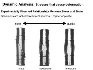
brittle. ductile. slate. sandstone. limestone. Dynamic Analysis: Stresses that cause deformation. Experimentally Observed Relationships Between Stress and Strain. Specimens are jacketed with weak material - copper or plastic. slate. sandstone. limestone.

E N D
brittle ductile slate sandstone limestone Dynamic Analysis: Stresses that cause deformation Experimentally Observed Relationships Between Stress and Strain Specimens are jacketed with weak material - copper or plastic.
slate sandstone limestone Specimens are drilled out cores that are ‘machined’ to have perfectly parallel and smooth ends. They are then carefully measured to determine their initial length (lo) and diameter (to get initial cross-sectional area, Ao)
Biaxial Test Rig Experiments are carried out in steel pressure vessels. Confining pressure (s2 = s3) is often supplied by fluid that surrounds the specimen. Temperature can be varied. Pore-fluid pressure can also be varied.
Types of Tests • Axial compression - either unconfined or confined. Results in length-parallel shortening. • Triaxial - specimen is subjected to 3 different loads (difficult), one may be tensile. • Tensile strength - specimen is pulled (rare).
s1 Fluid supplies confining pressure (s2 = s3) s2 = s3 s2 = s3 s1
Brazilian Test Axial splitting simulates tension
Results in length-parallel shortening. Vertical compressive stress (parallel to core) is taken to a higher level than the horizontal compressive stresses (confining pressure).
Results in length-parallel shortening. Horizontal compressive stress, perpendicular to core (confining pressure) is taken to a higher level than the vertical compressive stresses (parallel to the core).
Instead of squeezing a rock sample, they are pulled apart. Called tensile strength test. The aim is to determine the smallest amount of stress that will cause the rock to fail in tension. Rocks are much weaker in tension.
The Donath deformation apparatus In a natural setting confining pressure is the pressure exerted by the weight of interconnected pore fluids (hydrostatic pressure) and the overlying rockmass (lithostatic pressure). Here it is supplied by pumping up hydrologic fluid pressure.
If we increase confining pressure the specimen simply gets smaller - decreases volume. Confining does not cause distortion of the sample. Once the appropriate level of confining pressure has been achieved, then we can apply the axial load.
Calculating Axial Stress What we know is the load or force that is being applied (F) and the cross sectional area of the (A). s = F / A We keep track of a pair of numbers: E = axial strain and s = axial stress plot them in x,y space (respectively).
Measuring Shortening e = Dl / landS = lf / lo Strain Rate = e = e / t Measuring Strain Rate . Generally there are 2 kinds of tests: Constant Strain Rate & Constant Stress
A Standard Axial Compression Test • Measure initial specimen length and diameter. • Transform load into stress and displacement into % strain. • Plot differential stress (diameter of the Mohr circle for stress) against % strain. • Differential stress:sd=s1 - s3 Elastic loading
A Standard Axial Compression Test • Subject rock samples to controlled loading under known conditions. • 2) Fracture strength of rocks provides insight for structural geology • Rock strengths are measured by subjecting cylindrical samples (small rock core) to an axial load, applied by a cylinder or hydraulic ram. • The confining pressure is applied radially around the side by a fluid that is isolated from the rock by a deformable rubber or copper jacket. Elastic loading
Elastic loading and hysteresis What is the state of stress on a Mohr diagram? The state of stress plots as a single point on the Mohr diagram, because the axial stress equals the confining pressure. Differential stress: sd = s1 - s3 The state of stress appears on the Mohr diagram as successively large circle, of diameter s3-s1, sharing on the confining pressure s3, as a common point.
Eventually the sample starts to deform plastically. Its elastic behavior is surpassed, and non-recoverable deformation begins to accumulate in the rock. Plastic deformation produces deformation in a rock without failure by rupture. The onset of plastic deformation begins when the stress-strain curve departs from the straight line elastic mode. Below its yield strength the rock behaves as an elastic solid. The point of departure from elastic behavior is called the elastic limit. Its value is known as yield strength.
Faulting finally takes place at about 120 MPa and the stress drops to zero. Some of the elastic energy is expended making the fracture, some in sound, some in the frictional heating due to sliding. When we remove the sample, we notice that the fracture lies about 24° to the axis of the cylinder.
Stress/Strain Test: 1) Brittle rocks first shorten a elastically during these tests. 2) Then they fail abruptly by discrete fractures. 3) Sometimes plastic deformation occurs before failure, called strain softening. Just prior to failure (faulting), what if we raised the confining pressure and repeated the experiment on the same sample? How would the limestone respond?
Stress/Strain Test: When the load is reapplied at to Point C, the elastic limit is greater than during the first test. The yield strength is also greater, because the original fabric of the rock was changed slightly by the plastic deformation. This rock has undergone strain hardening. The yield strength increases due to modification of original rock.
Applying more load, the limestone displays an increase of plastic behavior before fracturing, unlike the previous experiment. This accelerated plastic deformation is called strain softening, because less stress is required for each new increment of strain. Eventually the rock fractures, but the rupture strength is greater in this experiment. Rupture strength is the stress level of failure by fracturing. Rocks become stronger at higher levels of confining pressure.
Rocks also undergo greater plastic deformation at higher levels of confining pressure, with T and strain rate fixed.
Confining Pressure (or Temperature) Low High As confining pressure (depth) increases, deformation becomes less discrete, and more distributed.
We need greater differential stress levels (s1 - s3) to cause rupture or failure when the confining pressure is increased (s3). This forms the basis for the laws that describe the conditions under which rocks fail by fracturing and faulting.
Each sample as different confining pressures before failure. It becomes obvious that we need greater differential stress levels (s1 - s3) to cause rupture or failure when the confining pressure is increased (s3). This forms the basis for the laws that describe the conditions under which rocks fail by fracturing and faulting.
Confining pressure Increasing confining pressure on a rock affects its strength. The slope of this failure envelope is a function of the rock’s angle of internal friction
Lithology & Strength Competent (strong & deform in a brittle manner) & Incompetent (weak & deform in a ductile manner)
Limestone become progressively more ductile at higher confining pressures Confining pressure or s3 For a given rock, yield strength, rupture strength, and ductility have greater values with increasing confining pressures.
Effect of Pore-Fluid Pressure on Strength • Fluid pressure also affects the strength of a rock • Increase of fluid pressure can offset or partially offset the effects of confining pressure. • 2) High fluid pressure decreases the strength of a rock. Water trapped in sediments during deposition may be overpressurized by burial and loading. • So the pore fluid stress is greater than the hydrostatic stress at any given level in the crust. Pf = fluid pressure 4) Trapped fluids that are have high pressures from burial and compaction 5) New term Effective stress = confining pressure – fluid pressure. The net effect of confining pressure and fluid pressure. 6) Allows deeply buried rocks to deform as if they were deforming in a low confining pressure environment.
Effect of Temperature on Strength • An increase in temperature of a rock can also depress the yield strength of a rock. • 2) Igneous rocks are less affected by low temperature changes than sedimentary rocks. • 3) If heated sufficiently, rocks will deform in a plastic or viscous fashion.
Effect of Strain Rate on Strength • Rock strength also if affected by rate of which stress is applied. • A rock can deform plastically at very low levels of stress if the rate of loading is very slow. Time vs. rock strength. • 2) Difficult to observe in experiments. Compare to long distance runners. Fractures are easier, at low stresses if stress is applied over a long time period (e.g. training and competition) Increase of strain rate
Creep - strains that result from low differential stresses over a very long time Primary creep: is slightly delayed elastic strain - tapers off with time. Secondary creep: a steady state plastic defm. Where strain and loading time are linearly related. Tertiary creep: fatigue finally sets in and strain accelerates - leads to failure by rupture.
looks like Mohr space? Depending on friction and normal forces, pre-existing frxs can be re-activated. As it turns out, friction properties for most rocks are the same. Linear relation between normal and shear stresses required to overcome friction and initiate movement.
Elastic, plastic, and viscous models of rock deformation Most tests are conducted as axial compression, where rocks fail in brittle, semi-brittle, or ductile manner. Although brittle and ductile are useful terms, less delve into the interplay of stress and strain. We will discuss three basic models. Elastic behavior Think of springs under a truck. If we load a truck, the springs will shorten by a amount directly related to the magnitude of load. The relationship of the load of blocks to the displacement of the bed is an equation that describe a straight line. It works perfectly, whether one loads or unloads the truck.
Elastic, Plastic and Viscous Models of Rock Behavior Hooke’s Law s = Ee: stress is linearly related to strain by the constant E, known as Young’s modulus
Elastic, plastic, and viscous models of rock deformation Hookes Law This straight line relation between stress and strain is called Hookes law (e µ s). Add proportionality constant to get Hookes law: s = Ee strain (e) is linearly proportional to stress (s) where E = Young’s modulus E = s/e = stress/strain The value of E, or Young’s modulus describes the slope of a straight line, stress-strain curve. Stress and strain are directly and linearly related = the slope of the line.
Young’s Modulus - a measure of elastic stiffness “a spring constant” E = s/e = stress/strain an elastic modulus. Young’s modulus, How much stress is required to achieve a given amount of length-parallel elastic shortening of a rock.
Hookes Law and Youngs Modulus For Hookes law relations, we plot stress (s) versus strain (e). The slope of the straight line is a measure of stiffness of a rock. The higher the value, the stiffer the rock, given in units of stress (MPa), Think of Young’s modulus as an elastic modulus, that describes how much stress is required to achieve a given amount of length-parallel elastic shortening.
Significance of Young’s Modulus • The relations between stress and strain (E = s/e ). E, or Young’s modulus equals force per unit area divided by changes in line length (strain). • Use steel railroad track example. Changes of expansion with respect to changes in temperature (thermal expansion). Steel track expands with increasing temperatures. • 2) Its coefficient of linear thermal expansion (a = 11 x 10-6). Thus a track 30 m long at 0°C will become 0.013m (i.e., 1.3 cm) longer when the steel warms to a temperature of 40°C.
Young’s Modulus 3) The changes of track length may not be much (centimeters), but if we look up Young’s modulus for steel (E = 8.67x10⁷ N/m2) and 4) Calculate the stress and then the force (s = F/A), we get very high forces (29 tons). A track can not respond elastically to such forces, so it deforms. This was from thermal expansion, not tectonic deformation.
Poisson’s Ratio (n) Describes the relationship between lateral strain and longitudinal strain. • =elat / elong • , another elastic modulus. • Vertical loading will produce horizontal stresses because of the Poisson effect. • The degree to which a specimen will widen upon shortening is a function of it’s Poisson’s ratio. • s2 = s3 = (n / (1 - n)) s1 • For common rocks, Poisson’s ratio tends to be around n = 0.25
Poisson’s ratio, Greek letter nu (n). This describes the amount that a rock bulges as it shortens. The ratio describes the ratio of lateral strain to longitudinal strain: n = elat/elong Poisson’s ratio is unitless, since it is a ratio of extension. What does this ratio mean? Typical values for n are: Fine-grained limestone: 0.25 Apilite: 0.2 Oolitic limestone: 0.18 Granite: 0.11 Walcareous shale: 0.02 Biotite schist: 0.01
Young’s Modulus If we shorten a granite and measure how much it bulges, we see that we can shorten a granite, but it may not be compensated by an increase in rock diameter. So stress did not produce the expected lateral bulging. Somehow volume decreases and stress was stored until the rock exploded! Thus low values of Poisson’s ratio are significant. Typical values for n are: Fine-grained limestone: 0.25 Apilite: 0.2 Oolitic limestone: 0.18 Granite: 0.11 Walcareous shale: 0.02 Biotite schist: 0.01
Bulk and Shear Moduli Bulk modulus (K): K = Dhydrostatic stress / Ddilation Shear modulus (G): G =ss / g • The two other parameters that describe the elastic relationship between stress and strain are: • 1) bulk modulus (K): resistance that elastic solids to changes in volume. • Divide the change of hydrostatic pressure by the amount of dilation produced by pressure changes. • K = bulk modulus = hyrdostatic stress /dilation • 2) Shear modulus (G): resistance that elastic solids to shearing: • Divide shear stress (ss) by shear strain (g) • G = shear modulus = ss/g
Elastic Stress - Strain Equations Applies to very small deformations in rocks Given si, E and n - we can solve for the strains
Plastic Strain No strains, below its yield stress, then when this level is achieved, the body will strain plastically as long as the yield stress magnitude is maintained. If we begin to deform (push) an ideal plastic body, nothing happens until the yield stress is overcome. Strain accumulates with no increase in stress.
Viscous Strain Think of shock absorbers. Viscous bodies are fluids, similar to a shock absorber. Even a tiny amount of stress will produce flow. These flows are permanent and not recoverable. Even the smallest amount of stress will displace a piston within a shock cylinder. No yield stress must be overcome in viscous behavior.