Strategy and Analysis Using NPV
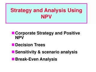
Strategy and Analysis Using NPV. Corporate Strategy and Positive NPV Decision Trees Sensitivity & scenario analysis Break-Even Analysis. How to Create Positive NPV. 1. Introduce a new product Apple’s introduction of the personal computer

Strategy and Analysis Using NPV
E N D
Presentation Transcript
Strategy and Analysis Using NPV • Corporate Strategy and Positive NPV • Decision Trees • Sensitivity & scenario analysis • Break-Even Analysis
How to Create Positive NPV 1. Introduce a new productApple’s introduction of the personal computer 2. Develop a core technologyHonda’s mastery of small-motor technology 3. Create a barrier to entryPolaroid’s patent on instant photographic film
How to Create Positive NPV 4. Introduce variations on existing productsChrysler’s introduction of the minivan 5. Create product differentiationCoca-Cola’s “It's the real thing” 6. Utilize organization innovationMotorola’s “just-in-time” inventory management
What does “risk” mean in capital budgeting? • Risk relates to uncertainty about a project’s future profitability. • Measured by sNPV, sIRR, beta. • Will taking on the project increase the firm’s and stockholders’ risk?
Is risk analysis based on historical data or subjective judgment? • Can sometimes use historical data, but generally cannot. • So risk analysis in capital budgeting is usually based on subjective judgments.
What three types of risk are relevant in capital budgeting? • Stand-alone risk • Corporate risk • Market risk
How is each type of risk measured, and how do they relate to one another? 1. Stand-Alone Risk: • The project’s risk if it were the firm’s only asset and there were no share-holders. • Ignores both firm and shareholder diversification. • Measured by the s or CV of NPV, IRR, or MIRR.
Probability Density Flatter distribution, larger s, larger stand-alone risk. NPV 0 E(NPV) Such graphics are increasingly used by corporations.
2. Corporate Risk: • Reflects the project’s effect on corporate earnings stability. • Considers firm’s other assets (diversification within firm). • Depends on: • project’s s, and • its correlation with returns on firm’s other assets. • Measured by the project’s corporate beta versus total corporate earnings.
Profitability Project X Total Firm Rest of Firm 0 Years 1. Project X is negatively correlated to firm’s other assets. 2. If r < 1.0, some diversification benefits. 3. If r = 1.0, no diversification effects.
3. Market Risk: • Reflects the project’s effect on a well-diversified stock portfolio. • Takes account of stockholders’ other assets. • Depends on project’s s and correlation with the stock market. • Measured by the project’s market beta.
How is each type of risk used? • Market risk is theoretically best in most situations. • However, creditors, customers, suppliers, and employees are more affected by corporate risk. • Therefore, corporate risk is also relevant.
Stand-alone risk is easiest to measure, more intuitive. • Core projects are highly correlated with other assets, so stand-alone risk generally reflects corporate risk. • If the project is highly correlated with the economy, stand-alone risk also reflects market risk.
Decision Trees • convenient way of representing sequential decisions over time • such decisions often arise when the uncertainty surrounding an investment can be reduced by some initial test marketing or preparing a feasibility study.
Decision Trees • EXAMPLE: Wild Kitty Drilling Co. owns some land in Alaska • Is not sure if there is oil on the land. • Exploratory well can be drilled today for £10 million • There is an 80% chance the well will come up dry.
Decision Trees • Whether the exploratory well is successful or not, production capacity can be installed in one year for £100 million • 10% discount rate is applied • If well is successful, annual cash flows would be £30 million • If unsuccessful, cash flow is £7.5 mil. • Invest in exploratory well?
Decision Trees (first part) Discount rate for both phases of the project = 10% Initial investment cost of exploratory well = £10M Subsequent investment Cost of production capacity installed in one year = £100M The well will produce the same amount of after-tax cash flow forever. This amount will not be known until after productive capacity is installed. Exploratory Productive Beginning of Well Capacity Returns on Investment Investment Investment (£10M) (£100M) 0 1 2
Decision Trees (second part) £50M (.25) E(CF) = £30M Invest £30M (.50) E(NPV) =£181.82M Success £10M (.25) (.2) Failure £30M (.1) (.8) E(CF) = £7.5M £15M (.3) £0 (.6) Don’t drill NPV = £0 Drill exploratory well Don’t invest NPV = £0 –£10M Invest E(NPV) = –£22.73M –£100M
Decision Trees (final part) Question 1. Should production begin in one year? E[NPVt=0|successful exploratory well] = (£30M/(.1) – £100M)/(1.1) = £181.82M > £0 ÞInvest E[NPVt=0|unsuccessful exploratory well] = (£7.5M/(.1) – £100M)/(1.1) = –£22.73M < £0 ÞDon’t invest Question 2. Should an exploratory well be dug today? E(NPV) = (.8)(£0) + (.2)(£181.82M) – £10M = £26.36M > £0 ÞInvest in exploratory well
What is sensitivity analysis? • Shows how changes in a variable such as unit sales affect NPV or IRR. • Each variable is fixed except one. Change this one variable to see the effect on NPV or IRR. • Answers “what if” questions, e.g. “What if sales decline by 30%?”
Sensitivity Analysis (first part) Under sensitivity analysis, one input is varied while all other inputs are assumed to meet their expectation. Suppose production is allowed to vary while all costs and sales prices are assumed equal to their expectation. Let annual cash flow given a successful exploratory well and starting in year two be given by: £30M £10M £50M .25 .50 .25 Project NPV evaluated at time 0 will be one of the following: £50M Þ NPV = (£50M/(.1) – £100M) / (1 + .1) = £363.64M £30M Þ NPV = (£30M/(.1) – £100M) / (1 + .1) = £181.82M £10M Þ NPV = (£10M/(.1) – £100M) / (1 + .1) = £0M The expected NPV at time zero based on the probabilities of each of these outcomes is again E[NPVt=0|successful exploratory well] = (.25)(£363.64M) + (.5)(181.82M) + (.25)(£0M) = £181.82M Slide T 8-3a
Sensitivity Analysis (final part) NPV £400M £300M £200M £100M £0 £10M £30M £50M .25 .50 .25 Annual cash flows given a successful exploratory well
Another Illustration Change from Resulting NPV (000s) Base Level Unit Sales Salvage k -30% -£ 36 £12 £34 -20 -19 13 28 -10 -2 14 21 0 (base) 15 15 15 +10 32 16 9 +20 49 17 3 +30 66 18 -2
NPV (000s) 70 Unit Sales Salvage 15 0 k % Change from base -40 -30 -20 -10 Base 10 20 30 Value
Results of Sensitivity Analysis • Steeper sensitivity lines show greater risk. Small changes result in large declines in NPV. • Unit sales line is steeper than salvage value or k, so NPV is more sensitive to changes in unit sales than in salvage value or k.
What are the weaknesses of sensitivity analysis? • Does not reflect diversification. • Says nothing about the likelihood of change in a variable, i.e., a steep sales line is not a problem if sales won’t fall. • Ignores relationships among variables.
Why is sensitivity analysis useful? • Gives some idea of stand-alone risk. • Identifies dangerous variables. • Gives some breakeven information.
What is scenario analysis? • Examines several possible situations, usually worst case, most likely case, and best case. • Provides a range of possible outcomes. • It is a “what if” analysis
Assume we know with certainty all variables except unit sales, which could range from 75,000 to 125,000. Scenario Probability NPV(000) Worst 0.25 -£27.8 Base 0.50 15.0 Best 0.25 57.8 E(NPV) = £15.0
sNPV E(NPV) £30.3 £15 CVNPV = = = 2.0. Standard Deviation sNPV = £30.3. Coefficient of Variation
If the firm’s average project has a CV of 1.25 to 1.75, is this a high-risk project? What type of risk is being measured? • Since CV = 2.0 > 1.75, this project hashigh risk. • CV measures a project’s stand-alone risk. It does not reflect firm or stockholder diversification.
Based on common sense, should the lemon project be highly correlated with the firm’s other assets? • Yes. Positively correlated. Economy and customer demand would affect all core products. • But each line could be more or less successful, so correlation less than +1.0.
Would correlation with the economy affect market risk? • Yes. • High correlation increases market risk (beta). • Low correlation lowers it.
With a 3% risk adjustment, should our project be accepted? • Project k = 10% + 3%= 13%. • That’s 30% above base k. • NPV = -£2,200, so reject.
What is a simulation analysis? • A computerized version of scenario analysis which uses continuous probability distributions of input variables. • Computer selects values for each variable based on given probability distributions. (Cont...)
NPV and IRR are calculated. • Process is repeated many times (1,000 or more). • End result: Probability distribution of NPV and IRR based on sample of simulated values. • Generally shown graphically.
Probability Density x x x x x x x x x x x x x x x x x x x x x x x x x x x x x x x x x x x x x x x x x x x x x x x x x x x x x x x x x x x x x x x x x x x x x x x 0 E(NPV) NPV Also gives sNPV, CVNPV, probability of NPV > 0.
What are the advantages of simulation analysis? • Reflects the probability distributions of each input. • Shows range of NPVs, the expected NPV, sNPV, and CVNPV. • Gives an intuitive graph of the risk situation.
What are the disadvantages of simulation? • Difficult to specify probability distributions and correlations. • If inputs are bad, output will be bad:“Garbage in, garbage out.” • May look more accurate than it really is. It is really a SWAG (“Scientific Wild A-- Guess”). (Cont...)
Sensitivity, scenario, and simulation analyses do not provide a decision rule. They do not indicate whether a project’s expected return is sufficient to compensate for its risk. • Sensitivity, scenario, and simulation analyses all ignore diversification. Thus they measure only stand-alone risk, which may not be the most relevant risk in capital budgeting.
Find the project’s market risk and cost of capital based on the CAPM, given these inputs: • Target debt ratio = 50%. • kd = 12%. • kRF = 10%. • Tax rate = 40%. • betaProject = 1.2. • Market risk premium = 6%.
Beta = 1.2, so project has more market risk than average. • Project’s required return on equity: ks = kRF + (kM - kRF)bp = 10% + (6%)1.2 = 17.2%. WACCp = wdkd(1 - T) + wceks = 0.5(12%)(0.6) + 0.5(17.2%) = 12.2%.
How does the project’s market risk compare with the firm’s overall market risk? • Project WACC = 12.2% versus company WACC = 10%. • Indicates that project’s market risk is greater than firm’s average project.
Is the project’s relative market risk consistent with its stand-alone risk? • Yes. Project CV = 2.0 versus 1.5 for an average project, which is consistent with project’s higher market risk.
Methods for Estimating a Project’s Beta 1. Pure play. Find several publicly traded companies exclusively in project’s business. Use average of their betas as proxy for project’s beta. Hard to find such companies.
2. Accounting beta.Run regression between project’s ROA and S&P index ROA. Accounting betas are correlated (0.5 - 0.6) with market betas. But normally can’t get data on new projects’ ROAs before the capital budgeting decision has been made.
Evaluating Risky Outflows • Company is evaluating two alternative waste disposal systems. Plan W requires more workers but less capital. Plan C requires more capital but fewer workers. • Both systems have 3-year lives. • The choice will have no impact on sales revenues, so the decision will be based on relative costs.
Year Plan W Plan C 0 (£500) (£1,000) 1 (500) (300) 2 (500) (300) 3 (500) (300) The two systems are of average risk, so WACC = 10%. Which to accept? PVCOSTSW = -£1,743. PVCOSTSC = -£1,746. W’s costs are slightly lower so pick W.
Now suppose Plan W is riskier than Plan C because future wage rates are difficult to forecast. Would this affect the choice? If we add a 3% risk adjustment to the 10% to get WACCW = 13%, W’s new PV would be: PVCOSTSW = -£1,681,which is < old PVCOSTSW = -£1,743. W now looks even better.
Plan W now looks better, but since it is riskier, it should look worse! • When costs are being discounted, we must use a lower discount rate to reflect higher risk. Thus, the appropriate discount rate would be 10% - 3% = 7%, making PVCOSTSW = -£1,812 > old -£1,743. • With risk adjustment, PVCOSTSW > PVCOSTSC, so now choose Plan C.