The Next-Generation Flexible Global Atmospheric Model
310 likes | 426 Vues
This presentation discusses the development of a next-generation, flexible global atmospheric model aimed at improving numerical weather prediction. Key features include the ability to test various dynamical cores, integration with Earth System Modeling Framework (ESMF), and a modular structure that facilitates the inclusion of different physics packages. The model is designed with modern coding practices, ensuring maintainability and usability. Current accomplishments, imminent steps, and challenges ahead, particularly in enhancing dynamics and physics, are addressed, paving the way for advancing operational weather forecasting.

The Next-Generation Flexible Global Atmospheric Model
E N D
Presentation Transcript
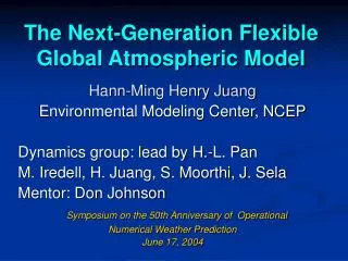
The Next-Generation Flexible Global Atmospheric Model Hann-Ming Henry Juang Environmental Modeling Center, NCEP Dynamics group: lead by H.-L. Pan M. Iredell, H. Juang, S. Moorthi, J. Sela Mentor: Don Johnson Symposium on the 50th Anniversary of Operational Numerical Weather Prediction June 17, 2004
Introduction • Reasons to develop new code • Flexible to test different dynamical cores • Develop to work with others, e.g. ESMF • Contents • Current design for flexibility • Current accomplishment • Immediate next steps • Future concerns
Rules of Code Design • Fortran 90 modules, libraries built. • C preprocessor for compiling options • NAMELIST for running-time dimension • Data structure for generalization • Pluggable physics packages • Possibly pluggable dynamics • ESMF-type for super-structure • Easy to maintain and friendly to use
Concept of Code Structure Super structure APIs Model layers APIs APIs : official ESMF; local ESMF; WRF API etc.
Element of Super Structure preprocessing package execution postprocessing
initial_prep (read namelist, allocation) initial_input (read input and data etc) atmos_initial initial_post (constant initialized) (allocate temporary spaces) model_prep atmos atmos_model model_integrate Model_post (deallocate temporary spaces) (prepare data for output) final_prep (write output or restart data) atmos_final final_output final_post (deallocation)
integrate_init ( prepare coefficients ) integrate_radiationpre (integrate_getgrid) integrate_radiation integrate_dynamicpre (integrate_getgrid) integrate_dynamics model_integrate - (integrate_getwave) integrate_dynamicsadj integrate_physicspre (integrate_getgrid) integrate_physics (integrate_getwave) integrate_physicsadj integrate_fine ( updating, time-filter etc)
dynamics_hybrid ( compute all values related to vertical coordinates etc ) integrate_dynamics - dynamics_nonadv ( compute all forcing except 3d advection ) dynamics_advect ( Eulerian or Lagrangian )
atmos_initial atmos2ocean_initial ocean_initial ocean2atmos_initial atmos_model atmos2ocean_trans atmos_ocean - ocean_model ocean2atmos_trans ocean2atmos_final ocean_final atmos2ocean_final atmos_final
Data Connection Variable structured data Structured Data Definition structured data Pass structured data, not by common block.
Generalized Variable Structure type atmos_dynamics_vars_type real*DYN_KIND, pointer :: valu(:,:,:) character*5 , pointer :: name(:) integer , pointer :: indx(:) integer len,lev, stp, num endtype atmos_dynamics_vars_type
Variable Definition type atmos_dynamics_defs_type character datatype*4 integer , pointer :: date(:) real fhour real , pointer :: dx(:) real , pointer :: dy(:) real , pointer :: ds(:) real , pointer :: sl(:) real , pointer :: si(:) integer numx,numy,nums integer numtracer,numdate,numwave endtype atmos_dynamics_defs_type
Running-time Dimension • Pass dimension and options through NAMELIST as &ATMOS_DEFINE datatype=’coef', wavenumber=64, layernumber=28, longitudenumber=108, latitudenumber=1, initialtime=0., finaltime=240., timestep=1800., filter=0.92, &END
Current Accomplishment • Implement all designs • Implement current operational dynamics and physics • Testing in three different platforms: ibm-sp, origin-o2k, pc-linux • Stable up to monthly integrations • Single and multiple tasks
Model Grid • Spectral model with spherical transform is suitable for spherical domain. • Reduce Gaussian grid (Williamson and Rosinski, 2000) • Reduce spherical transform (Juang 2004) • Reduce Gaussian grid • Reduce Legendre computation
Reduced (color) Full (black) Reduced - Full
Hybrid Parallel Computing • Code structure is the same for single and multi PE s • Only IO and spectral transform routine contain MPI related calls • 2D decomposition with 1D option • 2D can run more PE s • 1D is faster in vector machine • Multi-threads for outmost do-loop • Consider vector in inner do-loop • For different # of PEs without recompiling
24-h accumulated rainfall from FGM Contour intervals of 4x10⁻⁴ m
Next Steps • Generalized vertical coordinates • Implemented a generalized coordinates • Emphasized on sigma-theta coordinates • Current variables: U, V, T, P, and tracers • Comparisons forecast skills • Differences between sigma-p to sigma-theta • Differences from the operational one
P=0 q->infinite z=0 Isentropic dz/dt=0 P=P(q) z=qs/q P=Pq0 q=q0 sigma P=A(z)Pq0+B(z)Ps P=Ps z=1
Future Concerns • Improve Dynamics as well as Physics • Un-approximated primitive equation • Higher resolution physics • Improve Numerical Methods • Optimal between conservation and accuracy • Adopt multi-dynamical cores • Linkage to other components of earth models through ESMF
Model Equation • Nearly all global models are • Hydrostatic system • Diagnosis vertical momentum • Shallow-atmosphere assumption • Next generation could be years later • Very high resolution is expected • Hydrostatic is not valid • Full Coriolis effect • Deep atmosphere
Un-approximated Approach • From energy point of view • Energy=1/2[u(du/dt)+v(dv/dt)+w(dw/dt)] • Coriolis force and curvature terms are cancelled out • Cosine component of Coriolis force contributes to zonal vertical circulation • And r=a+z provides accurate curvature and displacement • Generalized vertical coordinates (Staniforth and Wood, 2003)
Full Coriolis Effect • Sine component of it modifies the flow pattern at middle- and high-latitudes • Cosine component of it modifies the vertical flow patterns at tropic and extra-tropic areas. • Coriolis force is approached to 10-4 from f and 10 from u, so it is about 10-3, and w is 10-2, 10% effect in w.
Not-shallow atmosphere For shallow assumption r = a (earth radius) For non-assumption r = a + z Not only affect gradients, curvature terms but also displacement by wind, since u = r cos d/dt and v = r d/dt For example, 50 m/s wind from100 hPa (20km) to 0.2 hPa (60km), errors in r=a are from 0.2 to above 1%, thus, errors in displacement after 10 days are from 20 km to 432 km.
Final Note With the combinations of • Sigma-theta coordinates to reduce the errors in vertical advection • Deep atmosphere to reduce the errors in stratospheric horizontal advection • Full Coriolis effect to have better vertical circulation along tropical areas The improvement on dynamical weather and climate forecasts can be expected.