Download
1 / 287
2.9k likes | 3.13k Vues
Relational Databases, Logic, and Complexity Phokion G. Kolaitis University of California, Santa Cruz & IBM Research-Almaden kolaitis@cs.ucsc.edu SELLC ‘10. What this course is about. Goals:

E N D
Relational Databases, Logic, and Complexity Phokion G. Kolaitis University of California, Santa Cruz & IBM Research-Almaden kolaitis@cs.ucsc.edu SELLC ‘10
What this course is about Goals: • Cover a coherent body of basic material in the foundations of relational databases • Prepare students for further study and research in relational database systems Overview of Topics: • Database query languages: expressive power and complexity • Relational Algebra and Relational Calculus • Conjunctive queries and homomorphisms • Recursive queries and Datalog • Selected additional topics: Bag Semantics, Inconsistent Databases Unifying Theme: The interplay between databases, logic, and computational complexity
The history of relational databases is the history of a scientific and technological revolution. The scientific revolution started in 1970 by Edgar (Ted) F. Codd at the IBM San Jose Research Laboratory (now the IBM Almaden Research Center) Codd introduced the relational data model and two database query languages: relational algebra and relational calculus. “A relational model for data for large shared data banks”, CACM, 1970. “Relational completeness of data base sublanguages”, in: Database Systems, ed. by R. Rustin, 1972. Edgar F. Codd, 1923-2003 Relational Databases: A Very Brief History
Relational Databases: A Very Brief History • Researchers at the IBM San Jose Laboratory embark on the System R project, the first implementation of a relational database management system (RDBMS) • In 1974-1975, they develop SEQUEL, a query language that eventually became the industry standard SQL. • System R evolved to DB2 – released first in 1983. • M. Stonebraker and E. Wong embark on the development of the Ingres RDBMS at UC Berkeley in 1973. • Ingres is commercialized in 1983; later, it became PostgreSQL, a free software OODBMS (object-oriented DBMS). • L. Ellison founds a company in 1979 that eventually becomes Oracle Corporation; Oracle V2 is released in 1979 and Oracle V3 in 1983. • Ted Codd receives the ACM Turing Award in 1981.
Relational Database Industry Today • According to Gartner, Inc., June 2007: “Worldwide relational database management systems (RDBMS) total software revenue totaled $15.2 billion in 2006, a 14.2 percent increase from 2005 revenue of $13.3 billion.” • In 2007, the total RDBMS software revenue increased to $17.1 billion (figures released in July 2008).
Database Research Today • A very vibrant community comprising several thousand researchers around the world. • Several major annual conferences in database research: • SIGMOD, PODS, VLDB, ICDE, EDBT, ICDT (top six). • Numerous other conferences and workshops. • Several major scholarly journals dedicated to database research: • ACM TODS, VLDB Journal, IEEE TKDE, … • Strong database research groups in academia around the world. • Several database research groups in industrial laboratories.
Database Management Systems A database management system (DBMS) provides support for: • At least one data model (a mathematical abstraction for representing data); • At least one high level data language (language for defining, updating, manipulating, and retrieving data); • Transaction management & concurrency control mechanisms; • Access control (limit access of certain data to certain users); • Resiliency (ability to recover from crashes).
Data Models and Data Languages • A data model is a mathematical formalism for describing and representing data. • A data model is accompanied by a data language that has two parts: a data definition language and a data manipulation language. • A data definition language (DDL) has a syntax for describing “database templates” in terms of the underlying data model. • A data manipulation language (DML) supports the following operations on data: • Insertion • Deletion • Update • Retrieval and extraction of data (query the data). • The first three operations are fairly standard. However, there is much variety on data retrieval and extraction (query languages).
The Relational Data Model (E.F. Codd – 1970) • The Relational Data Model uses the mathematical concept of a relation as the formalism for describing and representing data. • Question: What is a relation? • Answer: • Formally, a relation is a subset of a cartesian product of sets. • Informally, a relation is a “table” with rows and columns.
The Relational Data Model (E.F. Codd – 1970) • The Relational Data Model uses the mathematical concept of a relation as the formalism for describing and representing data. • Question: What is a relation? • Answer: • Formally, a relation is a subset of a cartesian product of sets. • Informally, a relation is a “table” with rows and columns. CHECKING-ACCOUNT Table
Basic Notions from Discrete Mathematics • A k-tuple is an ordered sequence of k objects (need not be distinct) • (2,0,1) is a 3-tuple; (a,b,a,a,c) is a 5-tuple, and so on. • If D1, D2, …, Dk are k sets, then the cartesian product D1£ D2 … £ Dk of these sets is the set of all k-tuples (d1,d2, …,dk) such that di 2 Di, for 1 · i · k. • Fact: Let |D| denote the cardinality (= # of elements) of a set D. Then |D1£ D2£ … £ Dk| = |D1|£ |D2| £ …£ |Dk|. • Example: If D1 = {0,1} and D2 ={a,b,c,d}, then |D1|£|D2| = 8. • Warning: Computing cartesian products is an expensive operation!
Basic Notions from Discrete Mathematics • A k-ary relation R is a subset of a cartesian product of k sets, i.e., • R µ D1£ D2£ … £ Dk. • Examples: • Unary R = {0,2,4,…,100} (R µ D) • Binary T = {(a,b): a and b have the same birthday} • Ternary S = {(m,n,s): s = m+n} • …
Relations and Attributes • Note: R µ D1£ D2£ … £ Dk can be viewed as a table with k columns Table S • In the relational data model, we want to have names for the columns; these are the attributes of the relation.
Relation Schemas and Relational Database Schemas • A k-ary relation schemaR(A1,A2,…,AK) is a set {A1,A2,…,Ak} of k attributes. • COURSE(course-no, course-name, term, instructor, room, time) • CITY-INFO(name, state, population) Thus, a k-ary relation schema is a “blueprint”, a “template” for some k-ary relation. • An instance of a relation schema is a relation conforming to the schema (arities match; also, in DBMS, data types of attributes match). • A relational database schema is a set of relation schemas Ri(A1,A2,…,Aki), for 1· i· m. • A relational database instance of a relational schema is a set of relations Ri each of which is an instance of the relation schema Ri, 1· i· m.
Relational Database Schemas - Examples • BANKING relational database schema with relation schemas • CHECKING-ACCOUNT(branch, acc-no, cust-id, balance) • SAVINGS-ACCOUNT(branch, acc-no, cust-id, balance) • CUSTOMER(cust-id, name, address, phone, email) • …. • UNIVERSITY relational database schema with relation schemas • STUDENT(student-id, student-name, major, status) • FACULTY(faculty-id, faculty-name, dpt, title, salary) • COURSE(course-no, course-name, term, instructor) • ENROLLS(student-id, course-no, term) • …
Schemas vs. Instances Keep in mind that there is a clear distinction between • relation schemas and instances of relation schemas and between • relational database schemas and relational database instances.
Programming Languages Paradigms There are two main paradigms of programming languages: imperative (or procedural) languages and declarative languages. • Imperative (Procedural) Languages: programs are expressed by specifying how the task is to be accomplished (sequence of operations). • FORTRAN, C, … • Declarative Languages: programs are expressed by specifying what has to be accomplished (as opposed to “how”). • LISP (functional programming), PROLOG (logic programming), …
Query Languages for the Relational Data Model Codd introduced two different query languages for the relational data model: • Relational Algebra, which is a procedural language. • It is an algebraic formalism in which queries are expressed by applying a sequence of operations to relations. • Relational Calculus, which is a declarative language. • It is a logical formalism in which queries are expressed as formulas of first-order logic. Codd’s Theorem: Relational Algebra and Relational Calculus are essentially equivalent in terms of expressive power. (but what does this really mean?)
Desiderata for a Database Query Language Desiderata: • The language should be sufficiently high-level to secure physical data independence, i.e., the separation between the physical level and the conceptual level of databases. • The language should have high enough expressive power to be able to pose useful and interesting queries against the database. • The language should be efficiently implementable to allow for the fast retrieval of information from the database. Warning: • There is a tension between the last two desiderata. • Increase in expressive power comes at the expense of efficiency.
Relational Algebra • Relational algebra strikes a good balance between expressive power and efficiency. • Codd’s key contribution was to identify a small set of basic operations on relations and to demonstrate that useful and interesting queries can be expressed by combining these operations. • Thus, relational algebra is a rich enough language, even though, as we will see later on, it suffers from certain limitations in terms of expressive power. • The first RDBMS prototype implementations (System R and Ingres) demonstrated that the relational algebra operations can be implemented efficiently.
The Five Basic Operations of Relational Algebra • Group I: Three standard set-theoretic binary operations: • Union • Difference • Cartesian Product. • Group II. Two special unary operations on relations: • Projection • Selection. • Relational Algebra consists of all expressions obtained by combining these five basic operations in syntactically correct ways.
Relational Algebra: Standard Set-Theoretic Operations • Union • Input: Two k-ary relations R and S, for some k. • Output: The k-ary relation R [ S, where R [ S = {(a1,…,ak): (a1,…,ak) is in R or (a1,…,ak) is in S} • Difference: • Input: Two k-ary relations R and S, for some k. • Output: The k-ary relation R - S, where R - S = {(a1,…,ak): (a1,…,ak) is in R and (a1,…,ak) is not in S} • Note: • In relational algebra, both arguments to the union and the difference must be relations of the same arity. • In SQL, there is the additional requirement that the corresponding attributes must have the same data type.
Relational Algebra: Standard Set-Theoretic Operations • Cartesian Product • Input: An m-ary relation R and an n-ary relation S • Output: The (m+n)-ary relation R £ S, where R £ S = {(a1,…,am,b1,…,bn): (a1,…am) is in R and (b1,…,bn) is in S} • Note: As stated earlier, |R£ S| = |R| £ |S|
The Projection Operator • Motivation: It is often the case that, given a table R, one wants to: • Rearrange the order of the columns • Suppress some columns • Do both of the above. • Fact: The Projection Operation is tailored for this task
The Projection Operation • Projection is a family of unary operations of the form ¼<attribute list> (<relation name>) • The intuitive description of the projection operation is as follows: • When projection is applied to a relation R, it removes all columns whose attributes do not appear in the <attribute list>. • The remaining columns may be re-arranged according to the order in the <attribute list>. • Any duplicate rows are also eliminated.
The Projection Operation - Example SAVINGS ¼cust-name,branch-name(SAVINGS)
More on the Syntax of the Projection Operation • In relational algebra, attributes can be referenced by position no. • Projection Operation: • Syntax:¼i1,…,im(R), where R is of arity k, and i_1, ….i_m are distinct integers from 1 up to k. • Semantics: ¼i1,…,im(R) = {(a1,…,am): there is a tuple (b1,…,bk) in R such that a1 = bi1, …, am = bim} • Example: If R is R(A,B,C,D), then ¼C,A (R) = ¼3,1(R)
The Selection Operation • Motivation: • Consider the table SAVINGS(branch-name, acc-no, cust-name, balance) • We may want to extract the following information from it: • Find all records in the Aptos branch • Find all records with balance at least $50,000 • Find all records in the Aptos branch with balance less than $1,000 • Fact: The Selection Operation is tailored for this task.
The Selection Operation • Selection is a family of unary operations of the form ¾£ (R), where R is a relation and £ is a condition that can be applied as a test to each row of R. • When a selection operation is applied to R, it returns the subset of R consisting of all rows that satisfy the condition £ • Question: What is the precise definition of a “condition”?
The Selection Operation • Definition: A condition in the selection operation is an expression built up from: • Comparison operators =, <, >,≠, ≤, ≥ applied to operands that are constants or attribute names or component numbers. • These are the basic (atomic) clauses of the conditions. • The Boolean logic operators Æ, Ç, : applied to basic clauses. • Examples: • balance > 10,000 • branch-name = “Aptos” • (branch-name = “Aptos”) Æ (balance < 1,000)
The Selection Operator • Note: • The use of the comparison operators <, >, ≤, ≥ assumes that the underlying domain of values is totally ordered. • If the domain is not totally ordered, then only= and ≠ are allowed. • If we do not have attribute names (hence, we can only reference columns via their component number), then we need to have a special symbol, say $, in front of a component number. Thus, • $4 > 100 is a meaningful basic clause • $1 = “Aptos” is a meaningful basic clause, and so on.
Relational Algebra • Definition: A relational algebra expression is a string obtained from relation schemas using union, difference, cartesian product, projection, and selection. • Context-free grammar for relational algebra expressions: E := R, S, … | (E1Ç E2) | (E1– E2) | (E1£ E2) | ¼L (E) |¾£(E), where • R, S, … are relation schemas • L is a list of attributes • £ is a condition.
Strength from Unity and Combination • By itself, each basic relational algebra operation has limited expressive power, as it carries out a specific and rather simple task. • When used in combination, however, the five relational algebra operations can express interesting and, quite often, rather complex queries. • Derived relational algebra operations are operations on relations that are expressible via a relational algebra expression (built from the five basic operators).
Intersection • Intersection • Input: Two k-ary relations R and S, for some k. • Output: The k-ary relation R Å S, where R Å S = {(a1,…,ak): (a1,…,ak) is in R and (a1,…,ak) is in S} • Fact: R Å S = R – (R – S) = S – (S – R) Thus, intersection is a derived relational algebra operation.
Natural Join • Fact: The most FAQs against databases involve the natural join operation ⋈. • Motivating Example: Given TEACHES(fac-name,course,term) and ENROLLS(stud-name,course,term), we want to obtain TAUGHT-BY(stud-name,course,term,fac-name) It turns out that TAUGHT-BY = ENROLSS ⋈ TEACHES
Natural Join Given TEACHES(fac-name,course,term) and ENROLLS(stud-name, course,term): To compute TAUGHT-BY(stud-name,course,term,fac-name) • ENROLLS £ TEACHES • ¾T.course = E.courseÆ T.term = E.term (ENROLLS £ TEACHES) • ¼stud-name,E.course,E.term,fac-name (¾T.course = E.course Æ T.term = E.term (ENROLLS £ TEACHES)) The result is ENROLLS ⋈ TEACHES.
Natural Join • Definition: Let A1, …, Ak be the common attributes of two relation schemas R and S. Then R ⋈ S = ¼<list> (¾R.A1=S.A1 Æ … Æ R.A1 = S.Ak (R£S)), where <list> contains all attributes of R£S, except for S.A1, …, S.Ak (in other words, duplicate columns are eliminated). • Algorithm for R ⋈S: For every tuple in R, compare it with every tuple in S as follows: • test if they agree on all common attributes of R and S; • if they do, take the tuple in R £ S formed by these two tuples, • remove all values of attributes of S that also occur in R; • put the resulting tuple in R ⋈ S.
Quotient (Division) • Motivating Example: Given ENROLLS(stud-name,course) and TEACHES(fac-name,course), find the names of students who take every course taught by V. Vianu. • Other Motivating Examples: • Find the names of customers who have an account in every branch of Wachovia in San Jose. • Find the names of Netflix customers who have rented every film in which Paul Newman starred. • These and other similar queries can be answered using the Quotient (Division) operation.
Quotient (Division) • Definition: Let R be a relation of arity r and let S be a relation of arity s, where r > s. The quotient (or division) R ÷ S is the relation of arity r – s consisting of all tuples (a1,…,ar-s) such that for every tuple (b1,…,bs) in S, we have that (a1,…,ar-s, b1,…,bs) is in R. • Example: Given ENROLLS(stud-name,course) and TEACHES(fac-name,course), find the names of students who take every course taught by V. Vianu. • Find the courses taught by V. Vianu ¼course (¾fac-name = “V. Vianu” (TEACHES)) • The desired answer is given by the expression: ENROLLS ÷ ¼course (¾fac-name = “V. Vianu” (TEACHES))
Quotient (Division) Fact: The quotient operation is expressible in relational algebra. Proof: For concreteness, assume that R has arity 5 and S has arity 2. Key Idea: Use the difference operation • R÷S = ¼1,2,3(R) – “tuples in ¼1,2,3(R) that do not make it to R÷S” • Consider the relational algebra expression (¼1,2,3(R)£S) – R. Intuitively, it is the set of all tuples that fail the test for membership in R÷S. Hence, • R÷S = ¼1,2,3(R) – ¼1,2,3( (¼1,2,3(R)£S) – R).
The Expressive Power of Relational Algebra • When combined together, the five basic relational algebra operations can express interesting and complex queries. • In particular, relational algebra can express: • The Intersection Operation • The Natural Join Operation • The Quotient Operation • ….
Independence of the Basic Relational Algebra Operations • Question: Are all five basic relational algebra operations really needed? Can one of them be expressed in terms of the other four? • Theorem: Each of the five basic relational algebra operations is independent of the other four, that is, it cannot be expressed by a relational algebra expression that involves only the other four. Proof Idea: For each relational algebra operation, we need to discover a property that is possessed by that operation, but is not possessed by any relational algebra expression that involves only the other four operations.
Independence of the Basic Relational Algebra Operations Theorem: Each of the five basic relational algebra operations is independent of the other four, that is, it cannot be expressed by a relational algebra expression that involves only the other four. Proof Sketch: (projection and cartesian product only) • Property of projection: • It is the only operation whose output may have arity smaller than its input. • Show, by induction, that the output of every relational algebra expression in the other four basic relational algebra is of arity at least as big as the maximum arity of its arguments. • Property of cartesian product: • It is the only operation whose output has arity bigger than its input. • Show, by induction, that the output of every relational algebra expression in the other four basic relational algebra is of arity at most as big as the maximum arity of its arguments. Exercise: Complete this proof.
Relational Algebra: Summary • When combined with each other, the five basic relational algebra operations can express interesting and complex queries (natural join, quotient, …) • The five basic relational algebra operations are independent of each other: none can be expressed in terms of the other four. • So, in conclusion, Codd’s choice of the five basic relational algebra operations has been very judicious.
Relational Completeness • Definition (Codd – 1972): A database query language L is relationally complete if it is at least as expressive as relational algebra, i.e., every relational algebra expression E has an equivalent expression F in L. • Relational completeness provides a benchmark for the expressive power of a database query language. • Every commercial database query language should be at least as expressive as relational algebra. • Exercise: Explain why SQL is relationally complete.
SQL vs. Relational Algebra Semantics of SQL via interpretation to Relational Algebra SELECT Ri1.A1, …, Rim.A.m FROM R1, …,RK = ¼Ri1.A1, …, Rim.A.m (¾ª (R1£ … £ RK)) WHERE ª
Relational Calculus • In addition to relational algebra, Codd introduced relational calculus. • Relational calculus is a declarative database query language based on first-order logic. • Relational calculus comes into two different flavors: • Tuple relational calculus • Domain relational calculus. We will focus on domain relational calculus. There is an easy translation between these two formalisms. • Codd’s main technical result is that relational algebra and relational calculus have essentially the same expressive power.
Propositional Logic (aka Boolean Logic) Reminder • Propositional variables: x, y, z, … • They take values 0 (True) and 1 (False). • Propositional connectives:Æ, Ç, :, ! • Propositional formulas: expressions built from propositional variables and propositional connectives • Syntax: := x, y, z, … | (Ã ÆÂ) | (ÃÇÂ) | :Ã | (Ã!Â) • Semantics: Truth-table semantics • Application: Propositional formulas express Boolean functions • (x Ç y) Æ (: x Ç: y) XOR-Gate • (x Æ y) Ç (x Æ z) Ç (y Æ z) Majority Gate
First-Order Logic - Motivation • First-Order Logic is a formalism for expressing properties of mathematical structures (graphs, trees, partial orders, …). • Example: Consider a graph G=(V,E) (nodes are in V, edges are in E) • There is a self-loop. • Every two nodes are connected via a path of length 2. • Every node has exactly three distinct neighbors. • There is a path of length 3 from node x to node y. • Node x has at least four distinct neighbors These and many other similar properties are expressible as formulas of first-order logic on graphs. • One of Codd’s key insights was that first-order logic can also be used to express relational database queries.
First-Order Logic • Question: What is First-Order Logic? • Answer: Informally, “ First-Order Logic = Propositional Logic + (9 and 8)”, where 9 and 8 range over possible values occurring in relations.