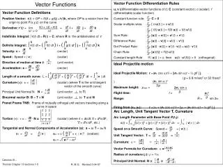
VECTOR FUNCTIONS

1. 13 VECTOR FUNCTIONS

2. VECTOR FUNCTIONS • Later in this chapter, we are going to use vector functions to describe the motion of planets and other objects through space. • Here, we prepare the way by developing the calculus of vector functions.

3. VECTOR FUNCTIONS 13.2 Derivatives and Integrals of Vector Functions • In this section, we will learn how to: • Develop the calculus of vector functions.

4. DERIVATIVES • The derivative r’ of a vector function is defined in much the same way as for real-valued functions.

5. DERIVATIVE Equation 1 • if this limit exists.

6. DERIVATIVE • The geometric significance of this definition is shown as follows.

7. SECANT VECTOR • If the points P and Q have position vectors r(t) and r(t + h), then represents the vector r(t + h) – r(t). • This can therefore be regarded as a secant vector.

8. DERIVATIVES • If h > 0, the scalar multiple (1/h)(r(t +h) – r(t)) has the same direction as r(t +h) – r(t). • As h → 0, it appears that this vector approaches a vector that lies on the tangent line.

9. TANGENT VECTOR • For this reason, the vector r’(t) is called the tangent vector to the curve defined by rat the point P, provided: • r’(t) exists • r’(t) ≠ 0

10. TANGENT LINE • The tangent lineto C at P is defined to be the line through P parallel to the tangent vector r’(t).

11. UNIT TANGENT VECTOR • We will also have occasion to consider the unit tangent vector:

12. DERIVATIVES • The following theorem gives us a convenient method for computing the derivative of a vector function r: • Just differentiate each component of r.

13. DERIVATIVES Theorem 2 • If r(t) = ‹f(t), g(t), h(t)› = f(t) i + g(t) j + h(t) k, where f, g, and h are differentiable functions, then: r’(t) = ‹f’(t), g’(t), h’(t)› = f’(t) i + g’(t) j + h’(t) k

14. DERIVATIVES Proof

15. DERIVATIVES Example 1 • Find the derivative of r(t) = (1 + t3) i + te–tj + sin 2t k • Find the unit tangent vector at the point where t = 0.

16. DERIVATIVES Example 1 a • According to Theorem 2, we differentiate each component of r: • r’(t) = 3t2i + (1 – t)e–tj + 2 cos 2t k

17. DERIVATIVES Example 1 b • As r(0) = i and r’(0) = j + 2k, the unit tangent vector at the point (1, 0, 0) is:

18. DERIVATIVES Example 2 • For the curve , find r’(t) and sketch the position vector r(1) and the tangent vector r’(1).

19. DERIVATIVES Example 2 • We have: • and

20. DERIVATIVES Example 2 • The curve is a plane curve. • Elimination of the parameter from the equations , y = 2 – t gives: • y = 2 – x2, x≥ 0

21. DERIVATIVES Example 2 • The position vector r(1) = i + j starts at the origin. • The tangent vector r’(1) starts at the corresponding point (1, 1).

22. DERIVATIVES Example 3 • Find parametric equations for the tangent line to the helix with parametric equations • x = 2 cos t y = sin t z =t • at the point (0, 1, π/2).

23. DERIVATIVES Example 3 • The vector equation of the helix is: r(t) = ‹2 cos t, sin t, t› • Thus, r’(t) = ‹–2 sin t, cos t, 1›

24. DERIVATIVES Example 3 • The parameter value corresponding to the point (0, 1, π/2) is t = π/2. • So, the tangent vector there is: r’(π/2) = ‹–2, 0, 1›

25. DERIVATIVES Example 3 • The tangent line is the line through (0, 1, π/2) parallel to the vector ‹–2, 0, 1›. • So, by Equations 2 in Section 12.5, its parametric equations are:

26. DERIVATIVES • The helix and the tangent line in the Example 3 are shown.

27. SECOND DERIVATIVE • Just as for real-valued functions, the second derivative of a vector function r is the derivative of r’, that is, r” = (r’)’. • For instance, the second derivative of the function in Example 3 is: r”(t) =‹–2 cos t, sin t, 0›

28. DIFFERENTIATION RULES • The next theorem shows that the differentiation formulas for real-valued functions have their counterparts for vector-valued functions.

29. DIFFERENTIATION RULES Theorem 3 • Suppose: • u and v are differentiable vector functions • c is a scalar • f is a real-valued function

30. DIFFERENTIATION RULES Theorem 3 • Then,

31. DIFFERENTIATION RULES Theorem 3

32. DIFFERENTIATION RULES • This theorem can be proved either: • Directly from Definition 1 • By using Theorem 2 and the corresponding differentiation formulas for real-valued functions

33. DIFFERENTIATION RULES • The proof of Formula 4 follows. • The remaining are left as exercises.

34. FORMULA 4 Proof • Let u(t) = ‹f1(t), f2(t), f3(t)› • v(t) = ‹g1(t), g2(t), g3(t)› • Then,

35. FORMULA 4 Proof • So, the ordinary Product Rule gives:

36. DIFFERENTIATION RULES Example 4 • Show that, if |r(t)| = c (a constant), then r’(t) is orthogonal to r(t) for all t.

37. DIFFERENTIATION RULES Example 4 • Since r(t) ∙r(t) = |r(t)|2 = c2and c2 is a constant, Formula 4 of Theorem 3 gives:

38. DIFFERENTIATION RULES • Thus, r’(t) ∙r(t) = 0 • This says that r’(t) is orthogonal to r(t).

39. DIFFERENTIATION RULES • Geometrically, this result says: • If a curve lies on a sphere with center the origin, then the tangent vector r’(t) is always perpendicular to the position vector r(t).

40. INTEGRALS • The definite integral of a continuous vector function r(t) can be defined in much the same way as for real-valued functions—except that the integral is a vector.

41. INTEGRALS • However, then, we can express the integral of r in terms of the integrals of its component functions f, g, and has follows. • We use the notation of Chapter 5.

42. INTEGRALS

43. INTEGRALS • Thus, • This means that we can evaluate an integral of a vector function by integrating each component function.

44. INTEGRALS • We can extend the Fundamental Theorem of Calculus to continuous vector functions: • Here, R is an antiderivative of r, that is, R’(t) = r(t). • We use the notation ∫ r(t)dtfor indefinite integrals (antiderivatives).

45. INTEGRALS Example 5 • If r(t) = 2 cos t i + sin t j + 2t k, then • where: • C is a vector constant of integration