Download
1 / 21
210 likes | 351 Vues
In this chapter, we explore the nature of random phenomena and their relationship with probability. We define key concepts such as outcomes, events, and the importance of independent trials. The Law of Large Numbers demonstrates how the long-run relative frequency of repeated events approaches the true probability. Additionally, we discuss formal probability requirements, including the complement rule and addition and multiplication rules for events. By adhering to established principles, we can accurately determine probabilities and understand their significance in everyday life.

E N D
From Randomness to ProbabilityChapter 14 Created by Jackie Miller, The Ohio State University
A random phenomenon is a situation in which we know what outcomes could happen, but we don’t know which particular outcome did or will happen. When dealing with probability, we will be dealing with many random phenomena. Dealing with Random Phenomena
The probability of an event is its long-run relative frequency. For any random phenomenon, each attempt, or trial, generates an outcome. Something happens on each trial, and we call whatever happens the outcome. An event consists of a combination of outcomes. Probability
When thinking about what happens with combinations of outcomes, things are simplified if the individual trials are independent. Basically, this means that the outcome of one trial doesn’t influence or change the outcome of another. For example, coin flips are independent. Probability (cont.)
The Law of Large Numbers (LLN) says that the long-run relative frequency of repeated independent events gets closer and closer to the true relative frequency as the number of trials increases. The Law of Large Numbers
For example, consider flipping a fair coin many, many times. The overall percentage of heads should settle down to about 50% as the number of outcomes increases. The Law of Large Numbers (cont.)
The common (mis)understanding of the LLN is that random phenomena are supposed to compensate some for whatever happened in the past. This is just not true. For example, when flipping a fair coin, if heads comes up on each of the first 10 flips, what do you think the chance is that tails will come up on the next flip? The Law of Large Numbers (cont.)
Thanks to the LLN, we know that relative frequencies settle down in the long run, so we can officially give the name probability to that value. Probabilities must be between 0 and 1, inclusive. A probability of 0 indicates impossibility. A probability of 1 indicates certainty. Probability Revisited
In everyday speech, when we express a degree of uncertainty without basing it on long-run relative frequencies, we are stating subjective or personal probabilities. Personal probabilities don’t display the kind of consistency that we will need probabilities to have, so we’ll stick with formally defined probabilities. Personal Probability
Two requirements for a probability: A probability is a number between 0 and 1. For any event A, 0 ≤ P(A) ≤ 1. Formal Probability
“Something has to happen rule”: The probability of the set of all possible outcomes of a trial must be 1. P(S) = 1 (S represents the set of all possible outcomes.) Formal Probability (cont.)
Complement Rule: Definition: The set of outcomes that are not in the event A is called the complement of A, denoted AC. The probability of an event occurring is 1 minus the probability that it doesn’t occur: P(A) = 1 – P(AC) Formal Probability (cont.)
Addition Rule: Definition: Events that have no outcomes in common (and, thus, cannot occur together) are called disjoint. Formal Probability (cont.)
Addition Rule: For two disjoint events A and B, the probability that one or the other occurs is the sum of the probabilities of the two events. P(AorB) = P(A) + P(B),provided that A and B are disjoint. Formal Probability (cont.)
Multiplication Rule: For two independent events A and B, the probability that both A and B occur is the product of the probabilities of the two events. P(AandB) = P(A) x P(B), provided that A and B are independent. Formal Probability (cont.)
Multiplication Rule: Two independent events A and B are not disjoint, provided the two events have probabilities greater than zero: Formal Probability (cont.)
Notation alert: In this text we use the notation P(A or B) and P(A and B). In other situations, you might see the following: P(AB) instead of P(A or B) P(AB) instead of P(A and B) Formal Probability - Notation
In most situations where we want to find a probability, we’ll use the rules in combination. A good thing to remember is that it can be easier to work with the complement of the event we’re really interested in. Putting the Rules to Work
Beware of probabilities that don’t add up to 1. Don’t add probabilities of events if they’re not disjoint. Don’t multiply probabilities of events if they’re not independent. Don’t confuse disjoint and independent—disjoint events can’t be independent. What Can Go Wrong?
Formal probabilities come to us compliments of the Law of Large Numbers: The long-run relative frequency of repeated independent events gets closer and closer to the true relative frequency as the number of trials increases. There are some basic principles of probabilities that we need to keep in mind. If we follow these principles and apply the correct rules, we will be able to find correct probabilities. Key Concepts