Realtime particle based fluid simulation
Realtime particle based fluid simulation. Stefan Auer. Contents. Introduction Motivation How to simulate fluids Related work Used techniques Fluid simulation Visualisation Conclusion. Fluids are ubiquitous parts of our environment

Realtime particle based fluid simulation
E N D
Presentation Transcript
Realtime particle basedfluid simulation Stefan Auer
Contents Introduction • Motivation • How to simulate fluids • Related work • Used techniques Fluid simulation Visualisation Conclusion
Fluids are ubiquitous parts of our environment (fluids include liquids and gases, but our focus is on liquids) I. Introduction 1) Motivation
realtime computer graphics tries to simulate the world believable dynamic fluids are rare in interactive applications CFD is a big topic, but mainly offline I. Introduction 1) Motivation
demand for fluids in interactive applications “Particle-Based Fluid Simulation for Interactive Applications” (2003) I. Introduction 1) Motivation
basis: Navier Stokes equations mostly result in non-linear PDEs -> numerical methods common: discretize (grid) + finite differences (or FEM) I. Introduction 2) How to simulate fluids
alternative to (Eulerian) grid based approach:particle based methods (Lagrangian) represent fluid as set of particles particle dynamics simulate fluid flow I. Introduction 2) How to simulate fluids
advantages: • equations and computations become simpler • no numerical diffusions • partly easier surface construction • fluid can spread freely in space I. Introduction 2) How to simulate fluids
chosen technique: smoothed particle hydrodynamics idea: particles distribute fluid properties in their neighbourhood done via smoothing functions I. Introduction 2) How to simulate fluids
SPH in general: • Developed by Gingold and Monaghan 1977 • and independently by Lucy (1977 too) • first usage: astronomy (LARGE scale gas-dynamics) • later used for liquids too (beach waves, sloshing tanks, ...) “SPH light” for interactive applications: • made public 2003 by Müller, Charypar, Gross: “Particle based fluid simulation for interactive appliactions” I. Introduction 3) Related work
following papers on realtime SPH: • Müller et al. 2004: “Interaction of fluids with deformable solids” • Kolb, Cuntz 2005: “Dynamic Particle Coupling for GPU-based Fluid Simulation” • Heinecke 2007: “Physikalische Rauchsimulation auf Partikelbasis in Echtzeit mit der PhysX-Engine“ I. Introduction 3) Related work
good visualisations are important (and complex) too: • Müller suggests 2003 direct point splatting of the particles or marching cubes • “Acceleration Techniques for GPU-based Volume Rendering” (2003 by Krüger, Westermann) among other things: isosurface ray-casting • Co et al. 2003: iso-splatting • Kipfer, Westermann 2003: “carpet based” river visualisation • Müller et al. 2007; “screen space meshes” I. Introduction 3) Related work
goal: simulation of water like liquids • believable movement • believable in optical appearance implemented fluid simulation in short: • same “lightweight” SPH model as Müller 2003 • neighbour search via dynamic grid • particles interact pair-wise • multi-core optimised I. Introduction 4) Used techniques
implemented visualisations in short: • sprite-based direct particle rendering • marching cubes • isosurface ray-tracing • based on isosurface ray-casting • simulates multiple reflections and refractions I. Introduction 4) Used techniques
Contents Introduction Fluid simulation • Basics of fluid mechanics • Basics of smoothed particle hydrodynamics • Particle based, mathematical model of fluid motion • Smoothing kernels • Basic simulation algorithm • Implementation • Environment and user interaction • Multithreading optimisation • Results • Further work and outlook • Visualisation • Conclusion
treat fluid as continuum every property has a defined value at each point in space mathematically: vector- or scalar fields fluid properties: • mass • “how much matter there is” • (mass-) density • “mass per volume” II. Fluid simulation 1) Basics of fluid mechanics
fluid properties continued: • pressure • scalar quantity • force in normal direction on a surface • velocity • vector quantity • measures how fast fluid passes a fixed point • influences most other quantities (advection) • relevant for viscosity forces II. Fluid simulation 1) Basics of fluid mechanics
fluid properties continued: • viscosity • compensates differences in flow velocity • comparable to friction • viscosity constant describes momentum transferbetween adjacent regions of different flow speed • viscosity force: tangential force on a surface • surface tension • property of the surface • describes size of forces that try to minimize the surface II. Fluid simulation 1) Basics of fluid mechanics
cause of surface tension (simple explanation) • surface molecules share cohesive forces with less neighbours II. Fluid simulation 1) Basics of fluid mechanics
now following: from Newtonian- to fluid mechanics “derivation” of the Navier Stokes equation • no mathematical derivation • only one particular equation variant discussed • goal: understand basic concepts, meaning and components of the equation basic statement: • “The Navier Stokes equation is the formulation of Newton’s second law of motion for fluids.” II. Fluid simulation 1) Basics of fluid mechanics
Newton’s second law of motion: in Newtonian mechanics usually interpretedfrom the Lagrangian point of view: • observer follows a moving object • with fluids: watch always the same “amount of fluid” alternative: Eulerian point of view • observe always the same point in space • with fluids: watched “amount of fluid” changes when fluid moves II. Fluid simulation 1) Basics of fluid mechanics
Eulerian vs. Lagrangian point of view: II. Fluid simulation 1) Basics of fluid mechanics
acceleration in Lagrangian point of view: • (simple) time derivative of velocity acceleration in Eulerian point of view: • convective derivative of velocity • convective derivative: Newton’s second law becomes: II. Fluid simulation 1) Basics of fluid mechanics
a certain volume element is watched mass in a volume is given by density -> split forces in fluid forces and external forces: II. Fluid simulation 1) Basics of fluid mechanics
external forces mainly gravity typically specified as acceleration (F=mg) mass still depends on density -> II. Fluid simulation 1) Basics of fluid mechanics
for the next step assume: • fluid is Newtonian • viscous stress proportional to velocity gradient • in common words: viscosity is a constant that doesn’tchange with different shear rates • fluid satisfies the incompressible flow condition • no sources or sinks in the velocity field • counter example: air that heats up • also flows of compressible fluid can satisfy the condition II. Fluid simulation 1) Basics of fluid mechanics
if all that’s the case, fluid forces can simply be split up: pressure force • depends only on pressure differences • points from high- to low pressure areas • -> the negative pressure gradient is what we want II. Fluid simulation 1) Basics of fluid mechanics
viscosity force • because of the incompressible flowcondition it becomes the simple term: • just believe it or see “Viscous fluid flow” (1999 by Papanastasiou et al.) for mathematical derivation • Laplacian operator measures how far a quantity is from the average around it • -> the force smoothes the velocity differences over time • this is what viscosity should do II. Fluid simulation 1) Basics of fluid mechanics
inserting viscosity force we arrive at Newton’s second law for fluids, the Navier Stokes equation: (more exactly: Navier Stokes momentum equationfor incompressible, Newtonian fluids) • which hopefully now is somehow understandable II. Fluid simulation 1) Basics of fluid mechanics
Contents Introduction Fluid simulation • Basics of fluid mechanics • Basics of smoothed particle hydrodynamics • Particle based, mathematical model of fluid motion • Smoothing kernels • Basic simulation algorithm • Implementation • Environment and user interaction • Multithreading optimisation • Results • Further work and outlook • Visualisation • Conclusion
SPH was developed for astrophysicalgas dynamics problems as in many other numerical solutions, values are interpolated from a discrete set of points SPH derives from the integral interpolation: • W: smoothing function (kernel) II. Fluid simulation 2) Basics of smoothed particle hydrodynamics
a word on the smoothing kernel: • “spreads a quantity in its surroundings” • is even (radial symmetric) • is normalised: • tends to become the deltafunction for h tending to zero(for h=0 the integral wouldreproduce A exactly) • for us: h = radius of support II. Fluid simulation 2) Basics of smoothed particle hydrodynamics
SPH is a Lagrangian method • moveable mass elements (particles)that carry properties • particle positions are the discrete setof interpolation points • interpolation integral becomes interpolation sum: • mass density coefficient appearsbecause each particle represents a volume: II. Fluid simulation 2) Basics of smoothed particle hydrodynamics
interesting example: • SPH interpolation applied to density • -> for SPH the density is simply thesmoothed mass of the particles in practical use not all particles must be evaluated • consider only particles that are within theradius of support (=h for us) II. Fluid simulation 2) Basics of smoothed particle hydrodynamics
advantage of SPH: simple derivatives • derivatives are very common in fluid equations • with SPH only the smoothing function has to be differentiated • the gradient therefore becomes: II. Fluid simulation 2) Basics of smoothed particle hydrodynamics
according to Müller this can be appliedfor the Laplacian too: this formulations are not “physically bullet-proof” • resulting equations can violate physical laws • -> correct them were necessary • also different definitions for SPH gradientand Laplacianexist in the literature II. Fluid simulation 2) Basics of smoothed particle hydrodynamics
Contents Introduction Fluid simulation • Basics of fluid mechanics • Basics of smoothed particle hydrodynamics • Particle based, mathematical model of fluid motion • Smoothing kernels • Basic simulation algorithm • Implementation • Environment and user interaction • Multithreading optimisation • Results • Further work and outlook • Visualisation • Conclusion
combine Navier Stokes equationwith basic SPH rules • discrete number of particles • particles carry only: • mass (constant and equal for all particles) • position • Velocity • all other quantities derived using SPHand basic physics equations II. Fluid simulation 3) Particle based, mathematical model of fluid motion
Eulerian models need equations for: • conservation of momentum (Navier Stokes) • conservation of mass(continuity equation) • conservation of energy (only sometimes) SPH needs only momentum equation • particle count and -masses constant -> mass constant II. Fluid simulation 3) Particle based, mathematical model of fluid motion
Eulerian models need convective derivative • because of advection SPH can use simple time derivative • advection implicit, because properties arecarried with the particles • -> replace convective derivative in N. S. equationwith time derivative • leads to momentum equation for a single particle: II. Fluid simulation 3) Particle based, mathematical model of fluid motion
particle acceleration therefore becomes simply: remember the SPH example for the density? all what’s missing is pressure- and viscosity force II. Fluid simulation 3) Particle based, mathematical model of fluid motion
pressure force • SPH rules would lead to the following pressure term: • unfortunately this force is not symmetric(think of two particles with different pressure) • fortunately a symmetric pendant is easy to find • use the arithmetic mean pressure: II. Fluid simulation 3) Particle based, mathematical model of fluid motion
pressure force continued • now we need the scalar pressure atthe particle’s position • Müller suggests the ideal gas state equation: • this introduces some drawbacks (compressibility i.e.) • we accept them for a simple simulation model II. Fluid simulation 3) Particle based, mathematical model of fluid motion
viscosity force • the SPH rule delivers: • again asymmetric , but again easy to symmetrise • viscosity depends only on velocity differences -> • the viscosity force in our model henceaccelerates each particle to meet the relativespeed of its environment II. Fluid simulation 3) Particle based, mathematical model of fluid motion
now we would be finished as we have equationsfor all what’s covered by the N. S. equation... ... but because we deal with much free surface,we will consider surface tension too II. Fluid simulation 3) Particle based, mathematical model of fluid motion
surface tension force • applies only to particles near the surface • pushes particles towards the inner of the fluid(-> negative surface normal) • higher surface curvature -> higher surface tension force the colour-field can deliver us all that • its gradient delivers the surface normaland is a measure for the surface-closeness • its Laplacian measures the surfacecurvature II. Fluid simulation 3) Particle based, mathematical model of fluid motion
in short the surface-tension term looks like this: • is near to zero for inner particles • -> surface tension only evaluated where itexceeds a threshold now our fluid model is complete II. Fluid simulation 3) Particle based, mathematical model of fluid motion
three different smoothing kernels are used: • poly6 • advantage: r appears only squared(no square roots) • used everywhere except for pressureand viscosity terms • spiky • gradient doesn’t vanish near the centre • used for pressure • viscosity • Laplacian stays positive everywhere • used for viscosity II. Fluid simulation 4) Smoothing kernels
used smoothing kernels: II. Fluid simulation 4) Smoothing kernels poly6 spiky viskosity
Contents Introduction Fluid simulation • Basics of fluid mechanics • Basics of smoothed particle hydrodynamics • Particle based, mathematical model of fluid motion • Smoothing kernels • Basic simulation algorithm • Implementation • Environment and user interaction • Multithreading optimisation • Results • Further work and outlook • Visualisation • Conclusion