Statistical Methods in Particle Physics Day 1: Introduction
Statistical Methods in Particle Physics Day 1: Introduction. 清华大学高能物理研究中心 2010 年 4 月 12—16 日. Glen Cowan Physics Department Royal Holloway, University of London g.cowan@rhul.ac.uk www.pp.rhul.ac.uk/~cowan. Outline of lectures. Day #1: Introduction Review of probability and Monte Carlo

Statistical Methods in Particle Physics Day 1: Introduction
E N D
Presentation Transcript
Statistical Methods in Particle PhysicsDay 1: Introduction 清华大学高能物理研究中心 2010年4月12—16日 Glen Cowan Physics Department Royal Holloway, University of London g.cowan@rhul.ac.uk www.pp.rhul.ac.uk/~cowan Statistical Methods in Particle Physics
Outline of lectures Day #1: Introduction Review of probability and Monte Carlo Review of statistics: parameter estimation Day #2: Multivariate methods (I) Event selection as a statistical test Cut-based, linear discriminant, neural networks Day #3: Multivariate methods (II) More multivariate classifiers: BDT, SVM ,... Day #4: Significance tests for discovery and limits Including systematics using profile likelihood Day #5: Bayesian methods Bayesian parameter estimation and model selection Statistical Methods in Particle Physics
Day #1: outline Probability and its role in data analysis Definition, interpretation of probability Bayes’ theorem Random variables and their properties A catalogue of distributions The Monte Carlo method Parameter estimation Method of maximum likelihood Method of least squares Statistical Methods in Particle Physics
Some statistics books, papers, etc. G. Cowan, Statistical Data Analysis, Clarendon, Oxford, 1998 see also www.pp.rhul.ac.uk/~cowan/sda R.J. Barlow, Statistics: A Guide to the Use of Statistical Methods in the Physical Sciences, Wiley, 1989 see also hepwww.ph.man.ac.uk/~roger/book.html L. Lyons, Statistics for Nuclear and Particle Physics, CUP, 1986 F. James., Statistical and Computational Methods in Experimental Physics, 2nd ed., World Scientific, 2006 S. Brandt, Statistical and Computational Methods in Data Analysis, Springer, New York, 1998 (with program library on CD) C. Amsler et al. (Particle Data Group), Review of Particle Physics, Physics Letters B667 (2008) 1; see also pdg.lbl.gov sections on probability statistics, Monte Carlo Statistical Methods in Particle Physics
Data analysis in particle physics Observe events of a certain type Measure characteristics of each event (particle momenta, number of muons, energy of jets,...) Theories (e.g. SM) predict distributions of these properties up to free parameters, e.g., a, GF, MZ, as, mH, ... Some tasks of data analysis: Estimate (measure) the parameters; Quantify the uncertainty of the parameter estimates; Test the extent to which the predictions of a theory are in agreement with the data (→presence of New Physics?) Statistical Methods in Particle Physics
A definition of probability Consider a set S with subsets A, B, ... Kolmogorov axioms (1933) Also define conditional probability: Statistical Methods in Particle Physics
Interpretation of probability I. Relative frequency A, B, ... are outcomes of a repeatable experiment cf. quantum mechanics, particle scattering, radioactive decay... II. Subjective probability A, B, ... are hypotheses (statements that are true or false) • Both interpretations consistent with Kolmogorov axioms. • In particle physics frequency interpretation often most useful, but subjective probability can provide more natural treatment of non-repeatable phenomena: systematic uncertainties, probability that Higgs boson exists,... Statistical Methods in Particle Physics
Bayes’ theorem From the definition of conditional probability we have and , so but Bayes’ theorem First published (posthumously) by the Reverend Thomas Bayes (1702−1761) An essay towards solving a problem in the doctrine of chances, Philos. Trans. R. Soc. 53 (1763) 370; reprinted in Biometrika, 45 (1958) 293. Statistical Methods in Particle Physics
B The law of total probability Consider a subset B of the sample space S, S divided into disjoint subsets Ai such that [i Ai = S, Ai B∩ Ai → → law of total probability → Bayes’ theorem becomes Statistical Methods in Particle Physics
Random variables and probability density functions A random variable is a numerical characteristic assigned to an element of the sample space; can be discrete or continuous. Suppose outcome of experiment is continuous value x →f(x) = probability density function (pdf) x must be somewhere Or for discrete outcome xi with e.g. i = 1, 2, ... we have probability mass function x must take on one of its possible values Statistical Methods in Particle Physics
Cumulative distribution function Probability to have outcome less than or equal to x is cumulative distribution function Alternatively define pdf with Statistical Methods in Particle Physics
Other types of probability densities Outcome of experiment characterized by several values, e.g. an n-component vector, (x1, ... xn) →joint pdf Sometimes we want only pdf of some (or one) of the components →marginal pdf x1, x2 independent if Sometimes we want to consider some components as constant →conditional pdf Statistical Methods in Particle Physics
Expectation values Consider continuous r.v. x with pdf f (x). Define expectation (mean) value as Notation (often): ~ “centre of gravity” of pdf. For a function y(x) with pdf g(y), (equivalent) Variance: Notation: Standard deviation: s ~ width of pdf, same units as x. Statistical Methods in Particle Physics
Covariance and correlation Define covariance cov[x,y] (also use matrix notation Vxy) as Correlation coefficient (dimensionless) defined as If x, y, independent, i.e., , then → x and y, ‘uncorrelated’ N.B. converse not always true. Statistical Methods in Particle Physics
Correlation (cont.) Statistical Methods in Particle Physics
Some distributions Distribution/pdf Example use in HEP Binomial Branching ratio Multinomial Histogram with fixed N Poisson Number of events found Uniform Monte Carlo method Exponential Decay time Gaussian Measurement error Chi-square Goodness-of-fit Cauchy Mass of resonance Landau Ionization energy loss Statistical Methods in Particle Physics
Binomial distribution Consider N independent experiments (Bernoulli trials): outcome of each is ‘success’ or ‘failure’, probability of success on any given trial is p. Define discrete r.v. n = number of successes (0 ≤n ≤ N). Probability of a specific outcome (in order), e.g. ‘ssfsf’ is But order not important; there are ways (permutations) to get n successes in N trials, total probability for n is sum of probabilities for each permutation. Statistical Methods in Particle Physics
Binomial distribution (2) The binomial distribution is therefore parameters random variable For the expectation value and variance we find: Statistical Methods in Particle Physics
Binomial distribution (3) Binomial distribution for several values of the parameters: Example: observe N decays of W±, the number n of which are W→mn is a binomial r.v., p = branching ratio. Statistical Methods in Particle Physics
Multinomial distribution Like binomial but now m outcomes instead of two, probabilities are For N trials we want the probability to obtain: n1 of outcome 1, n2 of outcome 2, nm of outcome m. This is the multinomial distribution for Statistical Methods in Particle Physics
Multinomial distribution (2) Now consider outcome i as ‘success’, all others as ‘failure’. → all ni individually binomial with parameters N, pi for all i One can also find the covariance to be represents a histogram Example: with m bins, N total entries, all entries independent. Statistical Methods in Particle Physics
Poisson distribution Consider binomial n in the limit →n follows the Poisson distribution: Example: number of scattering events n with cross section s found for a fixed integrated luminosity, with Statistical Methods in Particle Physics
Uniform distribution Consider a continuous r.v. x with -∞ < x < ∞ . Uniform pdf is: 2 N.B. For any r.v. x with cumulative distribution F(x), y = F(x) is uniform in [0,1]. Example: for p0→gg, Eg is uniform in [Emin, Emax], with Statistical Methods in Particle Physics
Exponential distribution The exponential pdf for the continuous r.v. x is defined by: Example: proper decay time t of an unstable particle (t = mean lifetime) Lack of memory (unique to exponential): Statistical Methods in Particle Physics
Gaussian distribution The Gaussian (normal) pdf for a continuous r.v. x is defined by: (N.B. often m, s2 denote mean, variance of any r.v., not only Gaussian.) Special case: m = 0, s2 = 1 (‘standard Gaussian’): If y ~ Gaussian with m, s2, then x = (y-m) /s follows (x). Statistical Methods in Particle Physics
Gaussian pdf and the Central Limit Theorem The Gaussian pdf is so useful because almost any random variable that is a sum of a large number of small contributions follows it. This follows from the Central Limit Theorem: For n independent r.v.s xi with finite variances si2, otherwise arbitrary pdfs, consider the sum In the limit n→ ∞, y is a Gaussian r.v. with Measurement errors are often the sum of many contributions, so frequently measured values can be treated as Gaussian r.v.s. Statistical Methods in Particle Physics
Central Limit Theorem (2) The CLT can be proved using characteristic functions (Fourier transforms), see, e.g., SDA Chapter 10. For finite n, the theorem is approximately valid to the extent that the fluctuation of the sum is not dominated by one (or few) terms. Beware of measurement errors with non-Gaussian tails. Good example: velocity component vx of air molecules. OK example: total deflection due to multiple Coulomb scattering. (Rare large angle deflections give non-Gaussian tail.) Bad example: energy loss of charged particle traversing thin gas layer. (Rare collisions make up large fraction of energy loss, cf. Landau pdf.) Statistical Methods in Particle Physics
Multivariate Gaussian distribution Multivariate Gaussian pdf for the vector are transpose (row) vectors, are column vectors, For n = 2 this is where r = cov[x1, x2]/(s1s2) is the correlation coefficient. Statistical Methods in Particle Physics
Chi-square (c2) distribution The chi-square pdf for the continuous r.v. z (z≥ 0) is defined by n = 1, 2, ... = number of ‘degrees of freedom’ (dof) For independent Gaussian xi, i = 1, ..., n, means mi, variances si2, follows c2 pdf with n dof. Example: goodness-of-fit test variable especially in conjunction with method of least squares. Statistical Methods in Particle Physics
Cauchy (Breit-Wigner) distribution The Breit-Wigner pdf for the continuous r.v. xis defined by (G = 2, x0 = 0 is the Cauchy pdf.) E[x] not well defined, V[x] →∞. x0 = mode (most probable value) G = full width at half maximum Example: mass of resonance particle, e.g. r, K*, f0, ... G = decay rate (inverse of mean lifetime) Statistical Methods in Particle Physics
Landau distribution For a charged particle with b = v /c traversing a layer of matter of thickness d, the energy loss D follows the Landau pdf: D + - + - b - + - + d L. Landau, J. Phys. USSR 8 (1944) 201; see also W. Allison and J. Cobb, Ann. Rev. Nucl. Part. Sci. 30 (1980) 253. Statistical Methods in Particle Physics
Landau distribution (2) Long ‘Landau tail’ →all moments ∞ Mode (most probable value) sensitive to b , →particle i.d. Statistical Methods in Particle Physics
Beta distribution Often used to represent pdf of continuous r.v. nonzero only between finite limits. Statistical Methods in Particle Physics
Gamma distribution Often used to represent pdf of continuous r.v. nonzero only in [0,∞]. Also e.g. sum of n exponential r.v.s or time until nth event in Poisson process ~ Gamma Statistical Methods in Particle Physics
Student's t distribution n = number of degrees of freedom (not necessarily integer) n = 1 gives Cauchy, n→ ∞ gives Gaussian. Statistical Methods in Particle Physics
Student's t distribution (2) If x ~ Gaussian with m = 0, s2 = 1, and z ~ c2 with n degrees of freedom, then t = x / (z/n)1/2 follows Student's t with n = n. This arises in problems where one forms the ratio of a sample mean to the sample standard deviation of Gaussian r.v.s. The Student's t provides a bell-shaped pdf with adjustable tails, ranging from those of a Gaussian, which fall off very quickly, (n → ∞, but in fact already very Gauss-like for n = two dozen), to the very long-tailed Cauchy (n = 1). Developed in 1908 by William Gosset, who worked under the pseudonym "Student" for the Guinness Brewery. Statistical Methods in Particle Physics
The Monte Carlo method What it is: a numerical technique for calculating probabilities and related quantities using sequences of random numbers. The usual steps: (1) Generate sequence r1, r2, ..., rm uniform in [0, 1]. (2) Use this to produce another sequence x1, x2, ..., xn distributed according to some pdf f (x) in which we’re interested (x can be a vector). (3) Use the x values to estimate some property of f (x), e.g., fraction of x values with a < x < b gives → MC calculation = integration (at least formally) MC generated values = ‘simulated data’ →use for testing statistical procedures Statistical Methods in Particle Physics
Random number generators Goal: generate uniformly distributed values in [0, 1]. Toss coin for e.g. 32 bit number... (too tiring). → ‘random number generator’ = computer algorithm to generate r1, r2, ..., rn. Example: multiplicative linear congruential generator (MLCG) ni+1 = (a ni) mod m , where ni = integer a = multiplier m = modulus n0 = seed (initial value) N.B. mod = modulus (remainder), e.g. 27 mod 5 = 2. This rule produces a sequence of numbers n0, n1, ... Statistical Methods in Particle Physics
Random number generators (2) The sequence is (unfortunately) periodic! Example (see Brandt Ch 4): a = 3, m = 7, n0 = 1 ← sequence repeats Choose a, m to obtain long period (maximum = m- 1); m usually close to the largest integer that can represented in the computer. Only use a subset of a single period of the sequence. Statistical Methods in Particle Physics
Random number generators (3) are in [0, 1] but are they ‘random’? Choose a, m so that the ri pass various tests of randomness: uniform distribution in [0, 1], all values independent (no correlations between pairs), e.g. L’Ecuyer, Commun. ACM 31 (1988) 742 suggests a = 40692 m = 2147483399 Far better algorithms available, e.g. TRandom3, period See F. James, Comp. Phys. Comm. 60 (1990) 111; Brandt Ch. 4 Statistical Methods in Particle Physics
The transformation method Given r1, r2,..., rn uniform in [0, 1], find x1, x2,..., xn that follow f (x) by finding a suitable transformation x (r). Require: i.e. That is, set and solve for x (r). Statistical Methods in Particle Physics
Example of the transformation method Exponential pdf: Set and solve for x (r). works too.) → Statistical Methods in Particle Physics
The acceptance-rejection method Enclose the pdf in a box: (1)Generate a random number x, uniform in [xmin, xmax], i.e. r1 is uniform in [0,1]. (2)Generate a 2nd independent random number u uniformly distributed between 0 and fmax, i.e. (3)If u < f (x), then accept x. If not, reject x and repeat. Statistical Methods in Particle Physics
Example with acceptance-rejection method If dot below curve, use x value in histogram. Statistical Methods in Particle Physics
Parameter estimation The parameters of a pdf are constants that characterize its shape, e.g. r.v. parameter Suppose we have a sample of observed values: We want to find some function of the data to estimate the parameter(s): ←estimator written with a hat Sometimes we say ‘estimator’ for the function of x1, ..., xn; ‘estimate’ for the value of the estimator with a particular data set. Statistical Methods in Particle Physics
Properties of estimators If we were to repeat the entire measurement, the estimates from each would follow a pdf: best large variance biased We want small (or zero) bias (systematic error): → average of repeated measurements should tend to true value. And we want a small variance (statistical error): →small bias & variance arein general conflicting criteria Statistical Methods in Particle Physics
An estimator for the mean (expectation value) Parameter: (‘sample mean’) Estimator: We find: Statistical Methods in Particle Physics
An estimator for the variance Parameter: (‘sample variance’) Estimator: We find: (factor of n-1 makes this so) where Statistical Methods in Particle Physics
The likelihood function Suppose the outcome of an experiment is: x1, ..., xn, which is modeled as a sample from a joint pdf with parameter(s) q: Now evaluate this with the data sample obtained and regard it as a function of the parameter(s). This is the likelihood function: (xi constant) If the xi are independent observations of x ~ f(x;q), then, Statistical Methods in Particle Physics
Maximum likelihood estimators If the hypothesized q is close to the true value, then we expect a high probability to get data like that which we actually found. So we define the maximum likelihood (ML) estimator(s) to be the parameter value(s) for which the likelihood is maximum. ML estimators not guaranteed to have any ‘optimal’ properties, (but in practice they’re very good). Statistical Methods in Particle Physics

