Download
1 / 59
590 likes | 764 Vues
Modeling the synergistic impacts of atmospheric and land-based influences on water quality and quantity in linked upland and estuarine ecosystems . Zong-Liang Yang (PI), David Maidment (co-PI), Paul Montagna (co-PI), James McClelland (co-PI), Hongjie Xie (co-PI)

E N D
Modeling the synergistic impacts of atmospheric and land-based influences on water quality and quantity in linked upland and estuarine ecosystems Zong-Liang Yang (PI), David Maidment (co-PI), Paul Montagna (co-PI), James McClelland (co-PI), Hongjie Xie (co-PI) Guo-Yue Niu, Seungbum Hong, Cédric David, Hae-Cheol Kim, Sandra Arismendez, Rae Mooney, Patty Garlough, Rachel Mills, Beibei Yu, Ling Lu, Almoutaz El Hassan 11-13 May 2010
Outline • Introduction • Models and tools • Climate change in Texas • Noah land surface model with multi-physics options • River network model (RAPID) • Statistical modeling of nutrient outflow • Estuary model • Summary and accomplishments • New IDS
Introduction: An incomplete water cycle • Atmosphere Land • To atmospheric scientists: • evapotranspiration (ET), space/time distribution; • runoff immediately lost to ocean, treated as a residual of P – ET • To hydrologists: • runoff, space/time; • river routing, ET is a residual (P – Runoff) • Land Oceans • To terrestrial hydrologists: figures mask oceans • To marine scientists: figures mask land
Modeling framework Zong-Liang Yang (UT Geological Sciences) Climate modeling Land surface modeling Hongjie Xie (UTSA Geological Sciences) Remote sensing analysis LULC, NEXRAD David Maidment (UT Civil Engineering) Hydrology, river routing Land/ocean coupling, BGC cycles Jim McClelland (UT Marine Science) Paul Montagna (TAMU Corpus Christi) Estuary ecology Coastal BGC
Framework for calculation Atmospheric Model or Dataset Land Surface Model Modeling across spatial and temporal scales: Globalregionalwatershedcoastal Current and future: interannual to hourly Vector River Network - High-Performance Computing River Network Model
Area of interest for integration with bays San Antonio Bay Mission Bay, Copano Bay and Aransas Bay
Guiding questions • What is the effect of global climate change on complex coastal environment processes? • What are the quantities of nutrient and organic matter export from land to sea? • How does the timing of export events influence ecosystem structure and productivity in coastal waters? • How do changes on land influence watershed export and ecosystem properties in coastal waters?
Precipitation gradient across Texas Texas is home to four of 10 largest cities in the nation. Chemical plants and oil refineries are located along the coast near Houston. Precipitation increases from semi-arid west to humid east. Temperature decreases from south to north.
Precipitation comparison Texas double peaks of monthly precipitation: spring, fall
Weather models and datasets WRF model Climate models NASA datasets (NLDAS, satellite datasets of land cover and change) Radar observations NEXRAD data
Land Surface Models forLand – atmosphere processes Noah model Noah is fully coupled with WRF in North America First version in 1999
NHDPlus – River and Catchment Network for the Nation Guadalupe and San Antonio Basins, TX Entire dataset Connectivity information 3 million river reaches 5,175 river reaches 26,000 km2 Integration of the National Hydrography Dataset, National Elevation Dataset and National Land Cover Dataset completed by EPA in 2006
River gages and dam operation data Historical and real-time measurements Dam operation data
Parallel computing for river flow mapping Parallel computer (UT’s Lonestar) Desktop computer • Today’s computers are as powerful as supercomputers ten years ago • Most computers come with multiple processors • High performance parallel computers are becoming increasingly accessible
Data • WCRP CMIP3 dataset • 16 global climate models • Three emission scenarios (A1B, A2, B1) • A1B 39 simulations • A2 37 simulations • B1 36 simulations • Precipitation and temperature (monthly) • Statistical downscaling with bias-correction
Projected probability distributions of surface temperature changes in the period of 2070–2099 relative to 1971-2000 means by different climate models over Texas
Projected monthly precipitation anomalies over individual five regions in Texas
Summary • Texas is getting warmer (2-5ºC by the end of this century); more warming in the north than in the south. • Overall decreasing trend of precipitation. Decreasing precipitation in the winter (5-15%), and increasing precipitation in the summer (5%). • We have downscaled precipitation (and other variables) at 3-hourly and fine-spatial scales for hydrological studies. • Bias correction is applied to precipitation before it is used to drive hydrological models.
Noah-MP with multi-physics options 1. Leaf area index (prescribed;predicted) 2. Turbulent transfer (Noah; NCAR LSM) 3. Soil moisture stress factor for transpiration (Noah;BATS;CLM) 4. Canopy stomatal resistance (Jarvis; Ball-Berry) 5. Snow surface albedo (BATS; CLASS) 6. Frozen soil permeability (Noah; Niu and Yang, 2006) 7. Supercooled liquid water (Noah; Niu and Yang, 2006) 8. Radiation transfer: Modified two-stream: Gap = F (3D structure; solar zenith angle; ...) ≤ 1-GVF Two-stream applied to the entire grid cell: Gap = 0 Two-stream applied to fractional vegetated area: Gap = 1-GVF 9. Partitioning of precipitation to snowfall and rainfall (CLM; Noah) 10. Runoff and groundwater: TOPMODEL with groundwater TOPMODEL with an equilibrium water table (Chen and Kumar, 2001) Original Noah scheme BATS surface runoff and free drainage More to be added Niu et al. (2010a,b)
Maximum # of Combinations 1. Leaf area index (prescribed; predicted) 2 2. Turbulent transfer (Noah; NCAR LSM) 2 3. Soil moisture stress factor for transp. (Noah; BATS; CLM) 3 4. Canopy stomatal resistance (Jarvis; Ball-Berry) 2 5. Snow surface albedo (BATS; CLASS) 2 6. Frozen soil permeability (Noah; Niu and Yang, 2006) 2 7. Supercooled liquid water (Noah; Niu and Yang, 2006) 2 8. Radiation transfer: 3 Modified two-stream: Gap = F (3D structure; solar zenith angle; ...) ≤ 1-GVF Two-stream applied to the entire grid cell: Gap = 0 Two-stream applied to fractional vegetated area: Gap = 1-GVF 9. Partitioning of precipitation to snow- and rainfall (CLM; Noah) 2 10. Runoff and groundwater: 4 TOPMODEL with groundwater TOPMODEL with an equilibrium water table (Chen and Kumar, 2001) Original Noah scheme BATS surface runoff and free drainage Niu et al. (2010a,b) 2x2x3x2x2x2x2x3x2x4 = 4608 combinations Ensemble-based process studies and quantification of uncertainties
Modeled Tskin (July 12th, 21:00 UTC, 2004) Niu et al. (2010b)
Modeled Leaf Area Index (LAI) and Green Vegetation Fraction (GVF) Niu et al. (2010b)
River network model: RAPID Routing Application for Parallel computatIon of Discharge
Framework for calculation Atmospheric Model or Dataset Land Surface Model Vector River Network - High-Performance Computing River Network Model
River network modeling • RAPID • Uses mapped rivers • Uses high-performance parallel computing • Computes everywhere including ungaged locations
Streamflow map 1) Optimize model parameters 2) Run model Flow calculated everywhere Guadalupe River at Victoria
Animation: flow map (Jan-Jun 2004) • 01/01/2004 – 06/30/2004 every 6 hours (RAPID computes 3-hourly) • 5,175 river reaches; 26,000 km2 • River model improves computations over lumped model, compared to observations at 36 gages Thank you to: Adam Kubach, Texas Advanced Computing Center
Transition of RAPID to other river basins • Learning RAPID • Compile and run for an existing case (0-1 months) if basic knowledge of Linux and Fortran • Adapting to new domain • Downloading NHDPlus data and preparing input files (2 weeks) • Downloading and processing USGS data (1 week) • Getting gridded runoff information
Water chemistry measurements and statistical modeling of nutrient outflow
San Antonio, Guadalupe, Mission and Aransas Rivers Watersheds
High resolution sampling • Sampling targeted to high flow events that potentially carry more nutrients
LOADEST Regression models MODEL 2 Ln(Conc) = a0 + a1 LnQ + a2 LnQ^2 where: Conc = constituent concentration LnQ = Ln(Q) - center of Ln(Q) MODEL 6 Ln(Conc) = a0 + a1 LnQ + a2 LnQ^2 + a3 Sin(2 pi dtime) + a4 Cos(2 pi dtime) where: Conc = constituent concentration LnQ = Ln(Q) - center of Ln(Q) dtime = decimal time - center of decimal time
Summary • Collected and analyzed 2-yr sampling data in Guadalupe, San Antonio, Mission, and Aransas rivers. • Noted that general patterns of DIN dilution and DON enrichment during storm flows are similar across all four rivers. • Major differences in nitrate concentrations among rivers (during low flows) reflect differences in anthropogenic nitrogen sources.
Study Area • Two River Basins • Guadalupe • San Antonio • Four HUCs in each basin • Guadalupe Estuary • Centrally located along Texas coast • Microtidal • Small bay area but large watershed relative to other Texas systems
A generic ecosystem model (3 components with 2 boundary conditions) Mass-balance model Two boundaries: LGRW & LSRW Three components: Nutrient (DIN) –Phytoplankton – Zooplankton Re-mineralization and implicit sinking (or horizontal exchange) were assumed to be 50%, respectively Δ=1 hr & RK 4th order scheme