A Model of Fluctuations
260 likes | 384 Vues
This text discusses the construction of a short-term economic fluctuations model, focusing on the Keynesian perspective. It emphasizes predetermined prices set by firms in the short run and the concept of planned aggregate expenditure (PAE) as key components influencing output. The model explores how consumer behavior, investment decisions, and government fiscal policy affect overall economic activity. It also examines the marginal propensity to consume (MPC) and its relationship with income changes, investment strategies, and the significance of inventory management within economic planning.

A Model of Fluctuations
E N D
Presentation Transcript
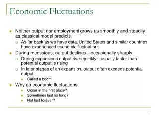
A Model of Fluctuations Here we begin to build a model of short term fluctuations in the economy around the long term trend.
A major assumption of our short term model is that in the short run prices of goods and services are predetermined and set by firms. The prices do not change for a while. Fluctuations in demand lead to changes in output, but not prices. Menu costs is a phrase we use to indicate the costly nature of changing prices in the short term. If you think about a restaurant, they have price printed on a menu and if they wanted to change prices to changing conditions of daily demand they would spend a lot on changing the menu often. By the way, the model we will study here is often called the Keynesian (rhymes with cane as in sugar cane, make it plural and add the name Ian – cane s Ian – Keynesian) model.
Planned Spending or Planned Aggregate Expenditure The authors note that the output in the economy is determined by the amount people plan to spend. What people plan to spend is called planned aggregate expenditure, or planned spending. Digress In the national economy we said that output could be split up into the components called consumption, investment, government spending and net exports (Y = C + I + G + NX). Part of investment is changes in inventory of the business community. Before I said investment is mainly new buildings, plant and equipment. While this is true, I now want to have you know about the changes in inventory as well.
To think about an example, say Coca Cola plans to add 100 cases of Coke to its inventory. Why? It wants to meet the needs of retailers and this is what it feels it needs. Associated with this planned addition to inventory, it has a plan for how much it will sell and it will produce accordingly. Say it plans on selling 1000 cases. So it will make 1100 cases. Now, if Coca Cola’s actual sales end up at 900 cases then 1) Actual sales (900) < planned sales (1000), and 2) Actual investment (200) > planned investment (100). Similarly, if actual sales are 1050 cases the 1) Actual sales (1050) > planned sales (1000), and 2) Actual investment (50) < planned investment (100).
Now let’s think about planned spending by households, businesses, governments and the rest of the world. We will assume that households, governments and the rest of the world can actually carry out their plans. So, for example, when households plan to consume a certain amount when the time comes they do what the plan. But, as we have seen with inventories, businesses can not always carry out their plan because folks may buy more or less than what the businesses planned and thus its actual inventory could be different than its plans. Next let’s turn to how each group goes about its planned spending.
Graph we use C, I, G, X 450 Read this part second. If on the 45 degree line we know the horizontal amount equals the vertical amount. Output or Income or RGDP Here we will use a graph that puts RGDP on the horizontal axis and C, I, G, and X components on the vertical axis. These vertical axis components are planned spending amounts! We can add them up if we want.
Consumption In the national economy we think the level of consumption expenditure depends on (among other things) income(RGDP). Say we have the following information: Income Consumption 1000 1600 2000 2200 3000 2800 If income rises then households will consume more. The reverse is true if income falls. Define MPC = marginal propensity to consume. The MPC is the number of pennies C changes for each $1 change in income.
Consumption - MPC The MPC is a fraction – the ratio of the change in consumption to the change in the income. Example: When income changes from 1000 to 2000 consumption changes from 1600 to 2200. The MPC = (2200-1600)/(2000-1000) = 600/1000 = .6 Note the MPC is the same all along the consumption function. In the graph on the next slide the slope of the consumption function is the MPC.
consumption in the graph C If income increases, we saw C will increase. We would move from point a to b, let’s say. We saw for every $ change in income, C changed by MPC. If from a to b income changed by 15 and MPC = .6, then C changed by ................? C b a income (did you get 9, it took me two tries to get it, but then again I am short and slow.)
Investment Investment is the amount of capital goods, buildings and changes in inventories business want to undertake in the current period. For now we focus on the planned investment and I will refer to it as Ip. For now we will assume all investment depends on factors other than income. For now we see it as a horizontal line representing a certain level of investment.
C+Ip C+I Putting the C and Ip lines together means at each income level add up C and Ip. C } Ip } C Ip
Government In our model the government can have an impact on the economy in two ways: 1) by affecting expenditures directly by its own expenditures, what will be called G, 2) by changing taxes and thus changing consumption C. Government expenditure in this model will not depend on the level of RGDP, but instead depend on the political process. Thus G will look much like I in the model, and can change if done so in the political arena. Note, if taxes change by some amount w, C changes in the opposite direction by MPC times w because taxes take away income from spending.
G G In the RGDP diagram the level of G will not depend on the level of income. In this regard it is similar to investment. The level of G can shift up or down, as we will see shortly. G1 income
C, I and G G, C, I The expenditure line is now the C+Ip+G line C1+Ip1+G1 G1 income
foreign sector X The foreign sector can be added to the model in much the same way that the government sector could be. The net exports does not change as the level of income changes. For ease I will use X instead of NX. X income
C, I, G, and X G, C, I, X C1+Ip1+G1 +X1 X1 income The planned expenditure line is now the C+Ip+G + X line
So, in the graph on the previous screen I have income on the horizontal axis. This is the actual level of output or income generated. The 45 degree line can help me translate these horizontal actual levels into vertical levels. The C + Ip + G + X line is the vertical planned amount of spending by the four sectors of the economy added up at each actual level of output. What level of actual output will result? Quick answer: The actual output level will be the one where planned output = actual output. Let’s see why this is the case by looking at other output levels.
Where will we be? G, C, I, X C1+Ip1+G1 +X1 Spending Income (Y1) income Y1 At Y1, planned spending is more than income. Essentially firms will see inventories falling to really low levels. This will have stores call for more production. Production and income will rise. (How can you spend more than amount in income? Borrow or spend down your savings – not a recommendation, just a statement.)
Where will we be? G, C, I, X Income (Y2) C1+I1+G1 +X1 Spending income Y2 At Y2, planned spending is less than income. Essentially stores will see inventories building up to really high levels. Stores will then call for less production. Production and income will fall. Why make stuff if no one is buying?
Where will we be? G, C, I, X Income (Y*) = C1+Ip1+G1 +X1 Spending This is called the spending balance point. income Ye At Ye, planned spending is equal to income. Essentially stores will see inventories be about right where they want them to be so it will seem demand is what they thought it would be. Production and income will stay right here.
You will notice on the previous screen that the C, Ip, G, X lines add up to C1 + Ip1 + G1 + X1 and thus we get income level Ye. But if C, I, G, or X should shift we would get a new point for income. On the next screen we will see government spending fall. Think about that. If G falls, goods the government used to buy would not be bought. Inventories would build up and we would expect firms to stop producing as much. Production and income (GDP) would fall. Silly story: When the President of the US has a dinner with foreign dignitaries, maybe the White House has two cokes available for each guest. Then there is a change in policy – only one coke per guest. Coke wouldn’t make as much and the production and income would fall. The fall is magnified when the government really cuts spending.
Say G falls G, C, I, X C1+Ip1+G1 +X1 (line was here) C1+Ip1+G2 +X1 (line falls to here) income Ye At Ye, spending is now more than income. Inventory will be too high (or demand is too low.) Production and income will fall.
Output gaps G, C, I, X Income (Y*) = PAE1 Spending income Y*1 Y*2 Y1 Expansionary gap Recessionary gap
Note on the previous screen that I have a line labeled PAE. This is just an easier way of typing C1 + Ip1 + G1 + X1. The actual economy will gravitate to Y1 (I dropped the e part of Ye). But, if the potential output level is at a point other than Y1 we will have an output gap. If the potential output is at Y*1, the actual output is above potential and we have an expansionary gap. Note at Y*1, Y*1 – Y1 < 0. If the potential output is at Y*2, the actual output is below potential and we have a recessionary gap. Note at Y*2, Y*2 – Y1 > 0.
How do we get to these gaps? Well, households control C, businesses control most of Ip (not the inventory part, as we said before), governments control G and the rest of the world controls X. Sometimes, folks have ideas that may mean the PAE line is not conducive to having the actual output occurring at the potential level. Fiscal policy Fiscal policy is a stabilization policy where the federal government influences the level of G or taxes (that affect C), or both. The idea is that perhaps the government can eliminate output gaps.
When there is a recessionary gap if the PAE line could be shifted up we could eliminate the gap. What do you think of this policy: have the president come on the TV and say to the people, “we have a recessionary gap and so if you just increase your spending we could eliminate the problem.” Maybe folks would respond. We Americans often rally when the country is in trouble. But maybe we can’t given out current budgets, taxes paid and the like. So, an example of a fiscal policy is for the government to cut our taxes and thus households would increase C and the PAE line would shift up. Another fiscal policy move would be for the government to just increase G (and not worry about changing taxes). Again PAE would shift up and the gap could be eliminated. The opposite fiscal policy measures would be good when we have an expansionary gap.