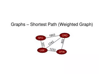
Graphs – Shortest Path (Weighted Graph)
Graphs – Shortest Path (Weighted Graph). 1843. ORD. SFO. 802. 1743. 337. 1233. LAX. DFW. Outline. The shortest path problem Single-source shortest path Shortest path on a directed acyclic graph (DAG) Shortest path on a general graph: Dijkstra’s algorithm. Outline.

Graphs – Shortest Path (Weighted Graph)
E N D
Presentation Transcript
Graphs – Shortest Path (Weighted Graph) 1843 ORD SFO 802 1743 337 1233 LAX DFW
Outline • The shortest path problem • Single-source shortest path • Shortest path on a directed acyclic graph (DAG) • Shortest path on a general graph: Dijkstra’s algorithm
Outline • The shortest path problem • Single-source shortest path • Shortest path on a directed acyclic graph (DAG) • Shortest path on a general graph: Dijkstra’s algorithm
Shortest Path on Weighted Graphs • BFS finds the shortest paths from a source node s to every vertex v in the graph. • Here, the length of a path is simply the number of edges on the path. • But what if edges have different ‘costs’? 7 1 v 5 v 2 s s 2 3
Weighted Graphs • In a weighted graph, each edge has an associated numerical value, called the weight of the edge • Edge weights may represent, distances, costs, etc. • Example: • In a flight route graph, the weight of an edge represents the distance in miles between the endpoint airports 849 PVD 1843 ORD 142 SFO 802 LGA 1205 1743 337 1387 HNL 2555 1099 1233 LAX 1120 DFW MIA
Shortest Path on a Weighted Graph • Given a weighted graph and two vertices u and v, we want to find a path of minimum total weight between u and v. • Length of a path is the sum of the weights of its edges. • Example: • Shortest path between Providence and Honolulu • Applications • Internet packet routing • Flight reservations • Driving directions 849 PVD 1843 ORD 142 SFO 802 LGA 1205 1743 337 1387 HNL 2555 1099 1233 LAX 1120 DFW MIA
Shortest Path: Notation • Input:
Shortest Path Properties Property 1 (Optimal Substructure): A subpath of a shortest path is itself a shortest path Property 2 (Shortest Path Tree): There is a tree of shortest paths from a start vertex to all the other vertices Example: Tree of shortest paths from Providence 849 PVD 1843 ORD 142 SFO 802 LGA 1205 1743 337 1387 HNL 2555 1099 1233 LAX 1120 DFW MIA
Shortest path trees are not necessarily unique Single-source shortest path search induces a search tree rooted at s. This tree, and hence the paths themselves, are not necessarily unique.
Optimal substructure: Proof • Lemma: Any subpath of a shortest path is a shortest path • Proof: Cut and paste.
Shortest path variants • Single-source shortest-paths problem: – the shortest path from s to each vertex v. • Single-destination shortest-paths problem: Find a shortest path to a given destination vertex t from each vertex v. • Single-pair shortest-path problem: Find a shortest path from u to v for given vertices u and v. • All-pairs shortest-paths problem: Find a shortest path from u to v for every pair of vertices u and v.
Negative-weight edges • OK, as long as no negative-weight cycles are reachable from the source. • If we have a negative-weight cycle, we can just keep going around it, and get w(s, v) = −∞ for all v on the cycle. • But OK if the negative-weight cycle is not reachable from the source. • Some algorithms work only if there are no negative-weight edges in the graph.
Cycles • Shortest paths can’t contain cycles: • Already ruled out negative-weight cycles. • Positive-weight: we can get a shorter path by omitting the cycle. • Zero-weight: no reason to use them assume that our solutions won’t use them.
Outline • The shortest path problem • Single-source shortest path • Shortest path on a directed acyclic graph (DAG) • Shortest path on a general graph: Dijkstra’s algorithm
Output of a single-source shortest-path algorithm • For each vertex v in V: • d[v] = δ(s, v). • Initially, d[v]=∞. • Reduce as algorithm progresses. But always maintain d[v] ≥ δ(s, v). • Call d[v] a shortest-path estimate. • π[v] = predecessor of v on a shortest path from s. • If no predecessor, π[v] = NIL. • π induces a tree — shortest-path tree.
Initialization • All shortest-path algorithms start with the same initialization: INIT-SINGLE-SOURCE(V, s) for each v in V do d[v]←∞ π[v] ← NIL d[s] ← 0
Relaxing an edge • Can we improve shortest-path estimate for v by first going to uand then following edge (u,v)? RELAX(u, v, w) if d[v] > d[u] + w(u, v) then d[v] ← d[u] + w(u, v) π[v]← u
General single-source shortest-path strategy • Start by calling INIT-SINGLE-SOURCE • Relax Edges Algorithms differ in the order in which edges are taken andhow many times each edge is relaxed.
Outline • The shortest path problem • Single-source shortest path • Shortest path on a directed acyclic graph (DAG) • Shortest path on a general graph: Dijkstra’s algorithm
Example 1. Single-Source Shortest Path on a Directed Acyclic Graph Basic Idea: topologically sort nodes and relax in linear order. Efficient, since δ[u] (shortest distance to u) has already been computed when edge (u,v) is relaxed. Thus we only relax each edge once, and never have to backtrack.
Example: Single-source shortest paths in a directed acyclic graph (DAG) • Since graph is a DAG, we are guaranteed no negative-weight cycles. • Thus algorithm can handle negative edges
Correctness of DAG Shortest Path Algorithm • Because we process vertices in topologically sorted order, edges of any path are relaxed in order of appearance in the path. • Edges on any shortest path are relaxed in order. • By path-relaxation property, correct.
Outline • The shortest path problem • Single-source shortest path • Shortest path on a directed acyclic graph (DAG) • Shortest path on a general graph: Dijkstra’s algorithm
Example 2. Single-Source Shortest Path on a General Graph (May Contain Cycles) This is fundamentally harder, because the first paths we discover may not be the shortest (not monotonic).
Dijkstra’s algorithm (E. Dijkstra,1959) • Applies to general, weighted, directed or undirected graph (may contain cycles). • But weights must be non-negative. (But they can be 0!) • Essentially a weighted version of BFS. • Instead of a FIFO queue, uses a priority queue. • Keys are shortest-path weights (d[v]). • Maintain 2 sets of vertices: • S = vertices whose final shortest-path weights are determined. • Q = priority queue = V-S. EdsgerDijkstra
We grow a “cloud” S of vertices, beginning with s and eventually covering all the vertices We store with each vertex v a label d(v) representing the distance of v from s in the subgraph consisting of the cloud S and its adjacent vertices At each step We add to the cloud S the vertex uoutside the cloud with the smallest distance label, d(u) We update the labels of the vertices adjacent to u Dijkstra’sAlgorithm: Operation 9 S s 1 4 11 7
Dijkstra’s algorithm • Dijkstra’s algorithm can be viewed as greedy, since it always chooses the “lightest” vertex in V − S to add to S.
Dijkstra’s algorithm: Analysis • Analysis: • Using minheap, queue operations takes O(logV) time
Example Key:
Djikstra’s Algorithm Cannot Handle Negative Edges 2 3 -2 1 y s x z
Correctness of Dijkstra’s algorithm • Loop invariant: d[v] = δ(s, v) for all v in S. • Initialization: Initially, S is empty, so trivially true. • Termination: At end, Q is empty S = V d[v] = δ(s, v) for all v in V. • Maintenance: • Need to show that • d[u] = δ(s, u) when u is added to S in each iteration. • d[u] does not change once u is added to S.
Correctness of Dijkstra’s Algorithm: Upper Bound Property • Upper Bound Property: • Proof: A valid path from s to v!
Correctness of Dijkstra’s Algorithm Optimal substructure property! Handled
? Correctness of Dijkstra’s algorithm • Loop invariant: d[v] = δ(s, v) for all v in S. • Maintenance: • Need to show that • d[u] = δ(s, u) when u is added to S in each iteration. • d[u] does not change once u is added to S.
Outline • The shortest path problem • Single-source shortest path • Shortest path on a directed acyclic graph (DAG) • Shortest path on a general graph: Dijkstra’s algorithm