Overview of Speech Recognition and Synthesis Course: Foundations and Applications
1.01k likes | 1.14k Vues
This course introduces speech recognition and synthesis, focusing on probabilistic models and language processing. Key topics include automatic speech recognition (ASR), speech-to-text, speech synthesis (TTS), and their practical applications such as dictation, telephony, and linguistic research. Historical insights into foundational models and early systems will set the context for current technologies. Emphasis is placed on supervised learning and search methodologies in TTS, alongside the exploration of language modeling and probability principles essential for understanding human speech processing.

Overview of Speech Recognition and Synthesis Course: Foundations and Applications
E N D
Presentation Transcript
LSA 352: Speech Recognition and Synthesis Dan Jurafsky Lecture 1: 1) Overview of Course 2) Refresher: Intro to Probability 3) Language Modeling IP notice: some slides for today from: Josh Goodman, Dan Klein, Bonnie Dorr, Julia Hirschberg, Sandiway Fong
Outline • Overview of Course • Probability • Language Modeling • Language Modeling means “probabilistic grammar”
Definitions • Speech Recognition • Speech-to-Text • Input: a wavefile, • Output: string of words • Speech Synthesis • Text-to-Speech • Input: a string of words • Output: a wavefile
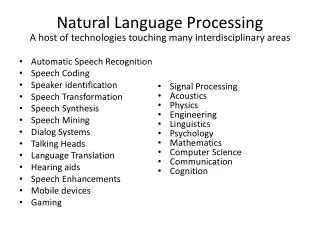
Automatic Speech Recognition (ASR)Automatic Speech Understanding (ASU) • Applications • Dictation • Telephone-based Information (directions, air travel, banking, etc) • Hands-free (in car) • Second language ('L2') (accent reduction) • Audio archive searching • Linguistic research • Automatically computing word durations, etc
Applications of Speech Synthesis/Text-to-Speech (TTS) • Games • Telephone-based Information (directions, air travel, banking, etc) • Eyes-free (in car) • Reading/speaking for disabled • Education: Reading tutors • Education: L2 learning
Applications of Speaker/Lg Recognition • Language recognition for call routing • Speaker Recognition: • Speaker verification (binary decision) • Voice password, telephone assistant • Speaker identification (one of N) • Criminal investigation
History: foundational insights 1900s-1950s • Automaton: • Markov 1911 • Turing 1936 • McCulloch-Pitts neuron (1943) • http://marr.bsee.swin.edu.au/~dtl/het704/lecture10/ann/node1.html • http://diwww.epfl.ch/mantra/tutorial/english/mcpits/html/ • Shannon (1948) link between automata and Markov models • Human speech processing • Fletcher at Bell Labs (1920’s) • Probabilistic/Information-theoretic models • Shannon (1948)
Synthesis precursors • Von Kempelen mechanical (bellows, reeds) speech production simulacrum • 1929 Channel vocoder (Dudley)
History: Early Recognition • 1920’s Radio Rex • Celluloid dog with iron base held within house by electromagnet against force of spring • Current to magnet flowed through bridge which was sensitive to energy at 500 Hz • 500 Hz energy caused bridge to vibrate, interrupting current, making dog spring forward • The sound “e” (ARPAbet [eh]) in Rex has 500 Hz component
History: early ASR systems • 1950’s: Early Speech recognizers • 1952: Bell Labs single-speaker digit recognizer • Measured energy from two bands (formants) • Built with analog electrical components • 2% error rate for single speaker, isolated digits • 1958: Dudley built classifier that used continuous spectrum rather than just formants • 1959: Denes ASR combining grammar and acoustic probability • 1960’s • FFT - Fast Fourier transform (Cooley and Tukey 1965) • LPC - linear prediction (1968) • 1969 John Pierce letter “Whither Speech Recognition?” • Random tuning of parameters, • Lack of scientific rigor, no evaluation metrics • Need to rely on higher level knowledge
ASR: 1970’s and 1980’s • Hidden Markov Model 1972 • Independent application of Baker (CMU) and Jelinek/Bahl/Mercer lab (IBM) following work of Baum and colleagues at IDA • ARPA project 1971-1976 • 5-year speech understanding project: 1000 word vocab, continous speech, multi-speaker • SDC, CMU, BBN • Only 1 CMU system achieved goal • 1980’s+ • Annual ARPA “Bakeoffs” • Large corpus collection • TIMIT • Resource Management • Wall Street Journal
State of the Art • ASR • speaker-independent, continuous, no noise, world’s best research systems: • Human-human speech: ~13-20% Word Error Rate (WER) • Human-machine speech: ~3-5% WER • TTS (demo next week)
LVCSR Overview • Large Vocabulary Continuous (Speaker-Independent) Speech Recognition • Build a statistical model of the speech-to-words process • Collect lots of speech and transcribe all the words • Train the model on the labeled speech • Paradigm: Supervised Machine Learning + Search
Unit Selection TTS Overview • Collect lots of speech (5-50 hours) from one speaker, transcribe very carefully, all the syllables and phones and whatnot • To synthesize a sentence, patch together syllables and phones from the training data. • Paradigm: search
Requirements and Grading • Readings: • Required Text: • Selected chapters on web from • Jurafsky & Martin, 2000. Speech and Language Processing. • Taylor, Paul. 2007. Text-to-Speech Synthesis. • Grading • Homework: 75% (3 homeworks, 25% each) • Participation: 25% • You may work in groups
Overview of the course • http://nlp.stanford.edu/courses/lsa352/
6. Introduction to Probability • Experiment (trial) • Repeatable procedure with well-defined possible outcomes • Sample Space (S) • the set of all possible outcomes • finite or infinite • Example • coin toss experiment • possible outcomes: S = {heads, tails} • Example • die toss experiment • possible outcomes: S = {1,2,3,4,5,6} Slides from Sandiway Fong
Introduction to Probability • Definition of sample space depends on what we are asking • Sample Space (S): the set of all possible outcomes • Example • die toss experiment for whether the number is even or odd • possible outcomes: {even,odd} • not {1,2,3,4,5,6}
More definitions • Events • an event is any subset of outcomes from the sample space • Example • die toss experiment • let A represent the event such that the outcome of the die toss experiment is divisible by 3 • A = {3,6} • A is a subset of the sample space S= {1,2,3,4,5,6} • Example • Draw a card from a deck • suppose sample space S = {heart,spade,club,diamond} (four suits) • let A represent the event of drawing a heart • let B represent the event of drawing a red card • A = {heart} • B = {heart,diamond}
Introduction to Probability • Some definitions • Counting • suppose operation oi can be performed in ni ways, then • a sequence of k operations o1o2...ok • can be performed in n1 n2 ... nk ways • Example • die toss experiment, 6 possible outcomes • two dice are thrown at the same time • number of sample points in sample space = 6 6 = 36
Definition of Probability • The probability law assigns to an event a nonnegative number • Called P(A) • Also called the probability A • That encodes our knowledge or belief about the collective likelihood of all the elements of A • Probability law must satisfy certain properties
Probability Axioms • Nonnegativity • P(A) >= 0, for every event A • Additivity • If A and B are two disjoint events, then the probability of their union satisfies: • P(A U B) = P(A) + P(B) • Normalization • The probability of the entire sample space S is equal to 1, I.e. P(S) = 1.
An example • An experiment involving a single coin toss • There are two possible outcomes, H and T • Sample space S is {H,T} • If coin is fair, should assign equal probabilities to 2 outcomes • Since they have to sum to 1 • P({H}) = 0.5 • P({T}) = 0.5 • P({H,T}) = P({H})+P({T}) = 1.0
Another example • Experiment involving 3 coin tosses • Outcome is a 3-long string of H or T • S ={HHH,HHT,HTH,HTT,THH,THT,TTH,TTTT} • Assume each outcome is equiprobable • “Uniform distribution” • What is probability of the event that exactly 2 heads occur? • A = {HHT,HTH,THH} • P(A) = P({HHT})+P({HTH})+P({THH}) • = 1/8 + 1/8 + 1/8 • =3/8
Probability definitions • In summary: Probability of drawing a spade from 52 well-shuffled playing cards:
Probabilities of two events • If two events A and B are independent • Then • P(A and B) = P(A) x P(B) • If flip a fair coin twice • What is the probability that they are both heads? • If draw a card from a deck, then put it back, draw a card from the deck again • What is the probability that both drawn cards are hearts? • A coin is flipped twice • What is the probability that it comes up heads both times?
How about non-uniform probabilities? An example • A biased coin, • twice as likely to come up tails as heads, • is tossed twice • What is the probability that at least one head occurs? • Sample space = {hh, ht, th, tt} (h = heads, t = tails) • Sample points/probability for the event: • ht 1/3 x 2/3 = 2/9 hh 1/3 x 1/3= 1/9 • th 2/3 x 1/3 = 2/9 tt 2/3 x 2/3 = 4/9 • Answer: 5/9 = 0.56 (sum of weights in red)
Moving toward language • What’s the probability of drawing a 2 from a deck of 52 cards with four 2s? • What’s the probability of a random word (from a random dictionary page) being a verb?
Probability and part of speech tags • What’s the probability of a random word (from a random dictionary page) being a verb? • How to compute each of these • All words = just count all the words in the dictionary • # of ways to get a verb: number of words which are verbs! • If a dictionary has 50,000 entries, and 10,000 are verbs…. P(V) is 10000/50000 = 1/5 = .20
Conditional Probability • A way to reason about the outcome of an experiment based on partial information • In a word guessing game the first letter for the word is a “t”. What is the likelihood that the second letter is an “h”? • How likely is it that a person has a disease given that a medical test was negative? • A spot shows up on a radar screen. How likely is it that it corresponds to an aircraft?
More precisely • Given an experiment, a corresponding sample space S, and a probability law • Suppose we know that the outcome is within some given event B • We want to quantify the likelihood that the outcome also belongs to some other given event A. • We need a new probability law that gives us the conditional probability of A given B • P(A|B)
An intuition • A is “it’s raining now”. • P(A) in dry California is .01 • B is “it was raining ten minutes ago” • P(A|B) means “what is the probability of it raining now if it was raining 10 minutes ago” • P(A|B) is probably way higher than P(A) • Perhaps P(A|B) is .10 • Intuition: The knowledge about B should change our estimate of the probability of A.
Conditional probability • One of the following 30 items is chosen at random • What is P(X), the probability that it is an X? • What is P(X|red), the probability that it is an X given that it is red?
S Conditional Probability • let A and B be events • p(B|A) = the probability of event B occurring given event A occurs • definition: p(B|A) = p(A B) / p(A)
A A,B B Conditional probability • P(A|B) = P(A B)/P(B) • Or Note: P(A,B)=P(A|B) · P(B) Also: P(A,B) = P(B,A)
Independence • What is P(A,B) if A and B are independent? • P(A,B)=P(A) ·P(B) iff A,B independent. P(heads,tails) = P(heads) · P(tails) = .5 · .5 = .25 Note: P(A|B)=P(A) iff A,B independent Also: P(B|A)=P(B) iff A,B independent
Bayes Theorem • Swap the conditioning • Sometimes easier to estimate one kind of dependence than the other
Summary • Probability • Conditional Probability • Independence • Bayes Rule
How many words? • I do uh main- mainly business data processing • Fragments • Filled pauses • Are cat and cats the same word? • Some terminology • Lemma: a set of lexical forms having the same stem, major part of speech, and rough word sense • Cat and cats = same lemma • Wordform: the full inflected surface form. • Cat and cats = different wordforms
How many words? • they picnicked by the pool then lay back on the grass and looked at the stars • 16 tokens • 14 types • SWBD: • ~20,000 wordform types, • 2.4 million wordform tokens • Brown et al (1992) large corpus • 583 million wordform tokens • 293,181 wordform types • Let N = number of tokens, V = vocabulary = number of types • General wisdom: V > O(sqrt(N))
Language Modeling • We want to compute P(w1,w2,w3,w4,w5…wn), the probability of a sequence • Alternatively we want to compute P(w5|w1,w2,w3,w4,w5): the probability of a word given some previous words • The model that computes P(W) or P(wn|w1,w2…wn-1) is called the language model. • A better term for this would be “The Grammar” • But “Language model” or LM is standard
Computing P(W) • How to compute this joint probability: • P(“the”,”other”,”day”,”I”,”was”,”walking”,”along”,”and”,”saw”,”a”,”lizard”) • Intuition: let’s rely on the Chain Rule of Probability
The Chain Rule of Probability • Recall the definition of conditional probabilities • Rewriting: • More generally • P(A,B,C,D) = P(A)P(B|A)P(C|A,B)P(D|A,B,C) • In general • P(x1,x2,x3,…xn) = P(x1)P(x2|x1)P(x3|x1,x2)…P(xn|x1…xn-1)
The Chain Rule Applied to joint probability of words in sentence • P(“the big red dog was”)= • P(the)*P(big|the)*P(red|the big)*P(dog|the big red)*P(was|the big red dog)
Very easy estimate: • How to estimate? • P(the|its water is so transparent that) P(the|its water is so transparent that) = C(its water is so transparent that the) _______________________________ C(its water is so transparent that)
Unfortunately • There are a lot of possible sentences • We’ll never be able to get enough data to compute the statistics for those long prefixes • P(lizard|the,other,day,I,was,walking,along,and,saw,a) • Or • P(the|its water is so transparent that)
Markov Assumption • Make the simplifying assumption • P(lizard|the,other,day,I,was,walking,along,and,saw,a) = P(lizard|a) • Or maybe • P(lizard|the,other,day,I,was,walking,along,and,saw,a) = P(lizard|saw,a)
Markov Assumption • So for each component in the product replace with the approximation (assuming a prefix of N) • Bigram version
Estimating bigram probabilities • The Maximum Likelihood Estimate