Download
1 / 52
550 likes | 886 Vues
Impact of Climate Change on Road Infrastructure. Mark Harvey mark.harvey@infrastructure.gov.au www.bitre.gov.au. Austroads project published in 2004. Austroads AP-R243/04 : Impact of Climate change on road infrastucture

E N D
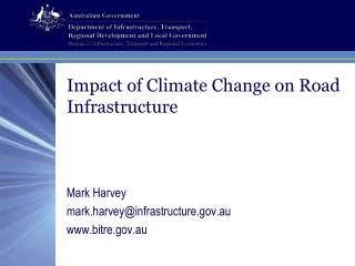
Impact of Climate Change on Road Infrastructure Mark Harvey mark.harvey@infrastructure.gov.au www.bitre.gov.au
Austroads project published in 2004 • Austroads AP-R243/04 : Impact of Climate change on road infrastucture • Downloadable for free from Austroads website, with volume of appendices AP-R243/04A • http://www.austroads.com.au • Also downloadable for free from BITRE website (main volume only) http:/www.bitre.gov.au • http://www.bitre.gov.au/publications/92/Files/climate_change.pdf
Project aims • assess likely local effects of climate change for Australia for the next 100 years, based on the best scientific assessment currently available • assess the likely impacts on patterns of demography and industry, and hence on the demand for road infrastructure • identify the likely effects on existing road infrastructure and potential adaptation measures in road construction and maintenance, and • report on policy implications arising from the findings. • Note: The project was not concerned with impacts of transport emissions on climate change.
Project structure • BITRE coordinated the project and prepared the Executive Summary, Introduction and the Policy Implications chapters. • The CSIRO Division of Atmospheric Research ran its global climate change models to produce forecasts of climate on a grid of about 50 kilometres up to 2100. • The resultant data was passed on to three consultants to assess its implications.
Project structure Emissions A2 scenario developed from population, energy and economic models Concentrations CO2, methane, sulphates, etc. from carbon cycle and chemistry models IPCC Global climate change Temperature, rainfall, etc. (200 – 400 km horizontal resolution) from Atmospheric-Ocean Global Climate Change Model Mark 2 Regional climate change Mountain & coastal effects, islands, extreme weather, surface properties, etc. (50 km horizontal resolution) from Conformal-Cubic model CSIRO ARRB, Monash University, ABARE, BITRE Impacts Population, industry, road pavements, salinity (various consultants)
Project structure continued • The Monash University Centre for Population and Urban Research investigated the likely effects on population settlement patterns and demographics. • ARRB Group used these population projections to forecast changes in road transport demand. • calculated changes to an index of climate from the CSIRO data • road demand and climatic indexes were together used in pavement deterioration models to predict the implications for pavement deterioration and maintenance expenditure needs.
Project structure continued • Australian Bureau of Agricultural and Resource Economics (ABARE) employed its hydrological–economic model of the Murray-Darling basin to forecast implications of climate change for salinity and agricultural production in the region, and related this to road infrastructure. • Multi-disciplinary project involving experts from a range of fields.
Project structure continued CSIRO: Regional climate change forecasts to 2100 Monash University Centre for Population and Urban Research: Impacts on population projections ABARE: Impacts on salinity and agriculture in Murray-Darling basin ARRB Group: Impacts on demand for roads ARRB Group: Impacts on road pavements BITRE: report and summary
Not covered in the study • Local flooding implications • requires a catchment hydrological model to predict flooding heights, durations and water velocities, and • an area topology model to relate flood heights to local road infrastructure. • Salinity and impacts of agricultural industries outside the Murray-Darling Basin • The CSIRO models do not forecast sea level rises or the likelihood of changes in storm activity.
Emissions forecasts • International Panel on Climate Change (IPCC) emissions scenario selected • ‘A2’ scenario • high scenario chosen to provide strong contrast with current conditions • predicated on global population of 15 billion in 2100 • rate of CO2 release grows, increasing to nearly fourfold by 2100.
IPCC emission scenarios A2 scenario (red line) used in this study.
CSIRO Atmospheric-Ocean Global Climate Change Model • global circulation model with atmospheric, oceanic, sea-ice and biospheric submodels • globe divided up into a grid comprised of 300 km squares • 9 layers of atmosphere, each block having parameters such as temperature, air pressure, wind velocity, water vapour content • 12 layers of ocean • time step of 30 minutes • run from 1870 to 2100 • suite of properties (temperature, moisture) saved for6-hourly intervals for the 230 years • took three months on a supercomputer
CSIRO Conformal-Cubic General Circulation Model • Results from global model used to ‘nudge’ more detailed model for Australia • wind speeds outside Australia adjusted to make consistent between models • grid of about 50 km squares for Australia and lower resolution for rest of the world (up to about 800 km for the other side of the globe)
Method of deriving detailed forecasts • outputs: monthly means of average, maximum and minimum temperatures, precipitation, solar radiation, potential and actual evaporation for each grid point • converted to • local temperature change per degree of global warming for temperature • percent for rainfall, radiation evaporation change per degree of global warming • used to derive forecast for any IPCC scenario for any grid point over the next 100 years.
Key findings: temperatures • average annual temperatures increase by 2⁰ to 6⁰C by 2100 • Tasmania coastal zones least affected, inland areas most affected • more extremely hot days and fewer cold days, for example • average number of summer days over 35⁰C in Melbourne to increase from 8 at present to 10-20 by 2070 • average number of winter days below 0⁰C in Canberra to drop from 44 at present to 6-38 by 2070
Average annual temperature: base (2000) and 2100 climate Base (2000) climate 2100 climate
Key findings: rainfall and evaporation • general reduction in rainfall except for the far north where there will be significant increases • where average rainfall decreases, more droughts • where average rainfall increases, more extremely wet years • in the north, more intense tropical cyclones, more severe oceanic storm surges, more frequent and heavier downpours • evaporation to increase over most of the country adding to moisture stress on plants and drought
Average annual rainfall: base (2000) and 2100 climate Base (2000) climate 2100 climate
Sea level rise • Not predicted in CSIRO modelling. • IPCC projects rise of 9 to 88 cm by 2100 • 0.8 to 8.0 cm per decade
Impact on population and settlement patterns: methodology • undertaken by Monash University Centre for Population and Urban Research (Dr Bob Birrell) • population projections developed for Australia as a whole, States and major metropolises (based on ABS mid-range projections supplemented by ANU demographic projection software). • adjustments made to the projections for the eight major metropolitan regions for climate change • using expert judgement supported by a comfort index (function of temperature and humidity). A comfortable climate is a major driver of internal migration.
Population base case: without climate change • total fertility rate will fall to 1.6 and net overseas migration 90,000 per year over the 21st century • total population 19.1m in 2000 to 27.3m in 2100 • greater concentration in four major metropolises: Sydney, Melbourne, Brisbane and Perth • other growth outside the four cities is in non-metropolitan Queensland and WA. • significant increase in share of population in Queensland • for planning purposes, need to take base case, then adjust for climate change
Population: climate change impacts • of the eight metropolitan regions assessed, only Darwin and Melbourne gain population from climate change • even though hotter, wetter Darwin less attractive, higher rainfall should promote agricultural production • but note the contrary view from the recent Northern Australia Land and Water Taskforce report: lack of suitable soils; high evaporation and lack of dam sites limits water storage • Losers: Adelaide (water supply), Cairns (less attractive climate) and Perth (water and climate) • coastal areas of NSW and Victoria more attractive climate • hotter, drier climate in inland areas will may have adverse impact on agriculture
Note: Climate change is not the most important influence on population patterns. • range of projections for 2100 compared with 2000 • without climate change: -63% Adelaide to 305% Darwin • with climate change: -50% Adelaide to 369% Darwin
Impact on road demand: Methodology • passenger and freight tasks considered separately • base-case forecasts developed • cars a function of population, per capita car ownership • freight a function of population, per capita freight, average payload (trend to larger vehicles) • converted to equivalent standard axel loads for pavement impacts • ARRB used a gravity model to estimate impacts of climate change on traffic. • If population at A increases by 100a% and population at B by 100b% due to climate change, then traffic between them increases by 100[(1+a)(1+b)-1]%.
Impact on road demand 2100: conclusions • 60% additional traffic (total vehicles passengers and freight) • dramatic increase in Queensland, moderate in Syd-Mel corridor, decline around Adelaide, increase in Perth urban only slight rise in Perth intercapital traffic • proportion heavy freight vehicles will rise from 12.1 to 13.9% • total road freight to rise by 112% from 2000 to 2100 • average payload to increase by 25%, most in next decade • equivalent standard axles per articulated truck to double due to higher mass limits • total ESA-kms on National Highway to rise by 230% • due to freight growth, higher mass limits and payloads
Impact on pavement performance: methodology • climate represented by ‘Thornthwaite moisture index’ • a function of precipitation, temperature and potential evapo-transpiration. Index varies from +100 on Cape Yorke Peninsula to -50 in central Australia. • used a National Highway System road database • pavement models estimate present value of life-cycle road agency costs (maintenance and rehabilitation) and road-user costs (travel time and vehicle operation) • select treatment options and timings to minimise present value of costs subject to specified constraints on maximum roughness and annual agency budgets.
Pavement Life Cycle Costing (PLCC) model • 60 year analysis period, 7% real discount rate • National Highway System split into 60 sections with similar climate characteristics, traffic levels, vehicle mixes and pavement characteristics • pavement deterioration a function of pavement age, cumulative equivalent standard axle loads, Thornthwaite index, and average annual maintenance expenditure.
HDM4 model • much more detailed pavement deterioration algorithm covering roughness, rutting, cracking, potholing, ravelling, strength etc and consequently much more detailed data requirements • case studies of 8 road segments analysed in detail • one segment from each state and territory located in or near a metropolitan area • data inputs that vary with climate are site-specific changes in Thornthwaite index, traffic levels and per cent heavy vehicles
Other points to note • Note: only trucks cause pavement wear, not cars • but cars impact on the models because increased roughness adds to road user costs for cars • Limitations • effects of floods, severe storms and sea-level rise not taken into account • no allowance for expansion of lane-kilometres • design pavement strengths assumed to remain unchanged • road agencies may not minimise present value of costs due to budget constraints causing maintenance to be deferred and higher than economically warranted maintenance standards in some areas for social and equity reasons
Thornthwaite moisture index: base (2000) and 2100 climates Base (2000) climate 2100 climate
Changes to Thornthwaite index • tendency to a drier climate overall (negative change in Thornthwaite Index) • central area of Australia relatively unchanged • localised areas where the changes are greatest include • south-west of Western Australia • north-east Victoria and southern NSW • south-west Tasmania • top-end Queensland.
Comparing optimal road agency costs • comparison is not with and without climate change • but 2000 traffic volumes and climate • with 2100 climate-adjusted traffic volumes and climate • Northern Territory and Queensland experience large increases • primarily due to population growth but wetter climate contributes. • South Australia declines due to smaller population and drier climate.
Maintenance: rehabilitation funding split • maintenance = routine and periodic maintenance (pothole patching, kerb and channel cleaning, surface correction, resealing) • rehabilitation = chipseal resheeting, asphalt overlays, stabilisation, pavement reconstruction • for Australia as a whole, no predicted change in 35:65 split • rehabilitation proportion to rise (maintenance proportion to fall) significantly for Tasmania • converse for WA • reflects differences in pavement age distributions and life times
HDM4 results: road agency costs • undiscounted total costs per kilometre over 20-year period • Virtually all the changes are from population growth leading to traffic increases, not climate change.
Impact on salinity in the Murray-Darling Basin: methodology • ABARE Salinity and Land-use Simulation Analysis (SALSA) model • network of land management units linked through overland and ground water flows • hydrological: rainfall, evapo-transpiration, surface water runoff, irrigation, ground water recharge/discharge rates, salt accumulation in streams and soil • climate projections incorporated by changing rainfall and evapo-transpiration • rate of flow of groundwater depends on ‘hydrolic gradients’ • very flat in lower parts of the catchment
Impact on salinity in the Murray-Darling Basin: methodology continued • land-use allocated to maximise economic return from use of agricultural land and irrigation water • relationship between yield loss and salinity for each agricultural activity • land-use can shift with changes in salinity and water availability • costs of salinity measured as reduction in economic returns
Catchments in the Murray Darling Basin covered by the SALSA model
Impact on salinity in the Murray-Darling Basin: Key findings
Impact on salinity in the Murray-Darling Basin: comparisons • area affected by high water tables • base case rise: from 1.1m hectares in 2000 to 5.3m hectares in 2100 • climate change: rise to 4.4m hectares in 2100 • climate change mitigates salinity problems but nowhere near sufficient to reverse the rising trend • net production revenue • base case: falls by 3% due to high water tables, shift from pasture to cropping • with climate change: falls by 11% due to reduced surface water flows, switching from irrigated to dryland activities • less demand for road transport
Impact on salinity in the Murray-Darling Basin: comparisons • higher water tables are bad for road pavements, but this is a problem in both the base and climate change scenarios • slightly less with climate change • reduced surface water flows make salt concentrations higher in rivers which reduces yields from irrigated production • and rusts steel reinforcing in concrete structures in riverine environments such as bridges and culverts.
Summing up: uncertainty • high level of uncertainty about • IPCC emissions forecasts • CSIRO estimates of climate impacts • consultants’ forecasts • uncertainties built upon uncertainties • numerical results are broad indicators that tell a story
Summing up: demand for roads • Higher car and truck traffic from population growth is the main driver of investment and maintenance needs for roads. • Large changes are forecast without climate change. • strong growth for SE Queensland, Cairns, Darwin, Brisbane, Sydney, Melbourne, Perth • decline for Adelaide and inland areas • Climate change adds to forecasts for Darwin and Melbourne and reduces forecasts for Adelaide, Perth and Cairns.
Summing up: road design and maintenance • less rainfall should slow pavement deterioration • but effects so small as to have negligible impact on costs • exception for far northern parts of Australia, which are forecast to become wetter. Capacities of culverts and waterways may prove inadequate. • sea-level rise a concern for low-lying roads in coastal areas • changed and frequencies of floods in some areas • requires modelling of individual catchments to forecast impacts
Overall conclusion • Changes affecting road infrastructure will occur regardless of climate change. • Climate change is just another factor in the mix, and usually not the most important. • The main impacts on road infrastructure may come from changes in flood heights and frequencies, and sea-level rise with storm surges, which were not addressed in detail in the project. • impacts vary greatly between locations
Subsequent research: ARRB: Climate change framework for Queensland Department of Main Roads in 2008 • report not published, but a summary is available in a conference paper by Evans, Tsolakis and Naude http://www.patrec.org/web_docs/atrf/papers/2009/1737_paper66-Evans.pdf (ATRF Conference 2009) • comprehensive list of potential impacts on road infrastructure and operations • detailed review of (short- and long-term) climate change forecasts for Queensland • framework to assess risks, and to assist in the planning of climate change mitigation and adaptation responses.