Distinct items:
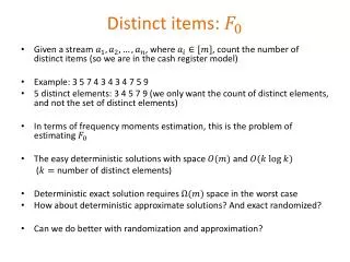
Distinct items: . Given a stream , where , count the number of distinct items (so we are in the cash register model) Example: 3 5 7 4 3 4 3 4 7 5 9 5 distinct elements: 3 4 5 7 9 (we only want the count of distinct elements, and not the set of distinct elements)

Distinct items:
E N D
Presentation Transcript
Distinct items: • Given a stream , where , count the number of distinct items (so we are in the cash register model) • Example: 3 5 7 4 3 4 3 4 7 5 9 • 5 distinct elements: 3 4 5 7 9 (we only want the count of distinct elements, and not the set of distinct elements) • In terms of frequency moments estimation, this is the problem of estimating • The easy deterministic solutions with space and ( number of distinct elements) • Deterministic exact solution requires space in the worst case • How about deterministic approximate solutions? And exact randomized? • Can we do better with randomization and approximation?
Counting distinct elements (Flajolet—Martin 1985) • Let be a random hash function: For each , value is uniformly distributed in • What is the relation between the minimum of and the number of distinct elements (We will do two proofs on the board, one algebraic and one pictorial) • Moreover, the variance can also be bounded via (Fun problem: I only know an algebraic proof for this, but there could be a pictorial one too given the suggestive-looking rhs)
Counting distinct elements First algorithm • Pick random hash function • Find the minimum of • Output • Estimator has high variance. Improving the estimator by averaging: Second algorithm • Run parallel independent copies of the first algorithm • Set ( is the estimate given by the th copy) • Return
Counting distinct elements • Space complexity of the first algorithm: To compute the minimum we just need to keep one real number in the memory. But need to limit precision • So the space requirement • Not quite: also need to account for the memory requirements for a random hash function • What property of random hash function did we really use?
Counting distinct elements • Pick from a 2-wise independent hash function family mapping for a prime ( is chosen large to reduce round off errors) • set of distinct elements • New estimator: • No longer clear that , but does provide useful information Lemma (probability is over the random choice of ) Proof (1) First, prove : Union bound
Counting distinct elements (2) Prove : • Define indicator if (this is the good event) otherwise • and so • We now upper bound by using the pairwise independence of the and Chebyshev’s inequality (proof on the board; also in the book page 297)
Boosting the success probability • Take the median of the means estimator • But doesn’t seem to give a -factor approximation approximation only within factors and • A related estimator [BJKST 2004]: • pairwise independent hash function family of functions of type • , so we can take , and have bits decription • So the probability that a random is injective is • Maintain the smallest hash values the th smallest hash value at the end of the stream The new estimator (BJKST estimator) is
Analyzing the BJKST estimator • Requirements to maintain the BJKST estimator: • Space • Update time • We assume (satisfied if true for ) • Recall that the set of distinct elements in the stream • We separately upper bound and using the Chebyshev inequality
Analyzing the BJKST estimator • I.e., contains at least elements less than (using ) • For , define if and otherwise • For • , , Chebyshev
Analyzing the BJKST estimator • Similarly, • Thus, • And now we can apply the median trick: Run parallel independent copies of the algorithm to compute and output their median TheoremThe output of the above algorithm is an -approximation of . It uses space and update time per streaming element Very powerful: A variant needs 128 bytes for all works of Shakespeare, ≈1/10 [Durand--Flajolet 2003] • What streaming model does the above algorithm require?
Counting distinct elements (strict turnstile model) • What about the strict turnstile model? • with integers • Frequency vector nonnegative • The previous algorithm requires cash register model • A different but closely related algorithm that works in the strict turnstile model • We will only give the basic idea and not the full details of the proof
Counting distinct elements (strict turnstile model) • set of distinct elements • First reduce the problem to its decision version: • Input: stream , parameters, and an additional parameter • Output: • YES if • NO if • Arbitrary otherwise • Solution of the decision version gives a solution of the general problem with a slight blow up in the space: • Run parallel versions of the decision problem with • A total of copies
Algorithm for the decision version of counting distinct elements Basic algorithm • Choose a random set by picking each element independently with probability : for all • Maintain • Output YES if else output NO
Decision version of counting distinct elements (analysis idea) LemmaFor and if if Proof
Full algorithm • Run independent parallel copies of the basic algorithm for sufficiently large constant : Sample independently, and maintain for each • if the ’th instance of the basic algorithm gives otherwise • Output YES (i.e. declare ) if • Output NO otherwise • An application of the Chernoff bound using the independence of the shows that this provides an -approximation • Space requirement? • Use 2-wise independent sampling to choose • Total space requirement is
Counting distinct elements • Why didn’t we just maintain whether or not ? • is a linear sketch • Allows for negative • So works in the (strict) turnstile model • The problem of computing is by now very well understood: space complexity with update time This is optimal up to constant factors [Kane et al. 2010]