Residence Time
Residence Time. Residence Time. Mean Water Residence Time (aka: turnover time, age of water leaving a system, exit age, mean transit time, travel time, hydraulic age, flushing time, or kinematic age) T = V / Q = turnover time or age of water leaving a system

Residence Time
E N D
Presentation Transcript
Residence Time • Mean Water Residence Time (aka: turnover time, age of water leaving a system, exit age, mean transit time, travel time, hydraulic age, flushing time, or kinematic age) • T= V/ Q = turnover time or age of water leaving a system • For a 10 L capped bucket with a steady state flow through of 2 L/hr, T = 5 hours • Assumes all water is mobile • Assumes complete mixing • For watersheds, we don’t know V or Q • Mean Tracer Residence Time (MRT) considers variations in flow path length and mobile and immobile flow
Residence and Geomorphology • Geomorphology controls fait of water molecule • Soils • Type • Depth • Bedrock • Permeability • Fracturing • Slope • Elevation
Transfer Function Models • Signal processing technique common in • Electronics • Seismology • Anything with waves • Hydrology
Transfer Function Models • Brief reminder of transfer function HYDROGRAPH model before returning to
flow Precipitation Hydrologic Model time time Hydrograph Modeling • Goal: Simulate the shape of a hydrograph given a known or designed water input (rain or snowmelt)
flow Precipitation Hydrologic Model time time Hydrograph Modeling: The input signal • Hyetograph can be • A future “design” event • What happens in response to a rainstorm of a hypothetical magnitude and duration • See http://hdsc.nws.noaa.gov/hdsc/pfds/ • A past storm • Simulate what happened in the past • Can serve as a calibration data set
flow Precipitation Hydrologic Model time time Hydrograph Modeling: The Model • What do we do with the input signal? • We mathematically manipulate the signal in a way that represents how the watershed actually manipulates the water • Q= f(P, landscape properties)
Hydrograph Modeling • What is a model? • What is the purpose of a model? • Types of Models • Physical • http://uwrl.usu.edu/facilities/hydraulics/projects/projects.html • Analog • Ohm’s law analogous to Darcy’s law • Mathematical • Equations to represent hydrologic process
Types of Mathematical Models • Process representation • Physically Based • Derived from equations representing actual physics of process • i.e. energy balance snowmelt models • Conceptual • Short cuts full physics to capture essential processes • Linear reservoir model • Empirical/Regression • i.e temperature index snowmelt model • Stochastic • Evaluates historical time series, based on probability • Spatial representation • Lumped • Distributed
Integrated Hydrologic Models Are Used toUnderstandandPredict(Quantify) the Movement of Water REW 2 REW 3 REW 4 REW 1 REW 5 p REW 7 REW 6 q Small Large Coarser Parametric Physics-Based Fine How ?Formalizationof hydrologic process equations Semi-DistributedModel DistributedModel Lumped Model e.g: Stanford Watershed Model e.g: HSPF, LASCAM e.g: ModHMS, PIHM, FIHM, InHM Process Representation: Predicted States Resolution: Data Requirement: Computational Requirement:
Hydrograph Modeling • Physically Based, distributed Physics-based equations for each process in each grid cell See dhsvm.pdf Kelleners et al., 2009 Pros and cons?
Hydrologic Similarity Models • Motivation: How can we retain the theory behind the physically based model while avoiding the computational difficulty? Identify the most important driving features and shortcut the rest.
TOPMODEL • Beven, K., R. Lamb, P. Quinn, R. Romanowicz and J. Freer, (1995), "TOPMODEL," Chapter 18 in Computer Models of Watershed Hydrology, Edited by V. P. Singh, Water Resources Publications, Highlands Ranch, Colorado, p.627-668. • “TOPMODEL is not a hydrological modeling package. It is rather a set of conceptual tools that can be used to reproduce the hydrological behaviour of catchments in a distributed or semi-distributed way, in particular the dynamics of surface or subsurface contributing areas.”
TOPMODEL • Surface saturation and soil moisture deficits based on topography • Slope • Specific Catchment Area • Topographic Convergence • Partial contributing area concept • Saturation from below (Dunne) runoff generation mechanism
TOPMODEL • Recognizes that topography is the dominant control on water flow • Predicts watershed streamflow by identifying areas that are topographically similar, computing the average subsurface and overland flow for those regions, then adding it all up. It is therefore a quasi-distributed model.
Key Assumptionsfrom Beven, Rainfall-Runoff Modeling • There is a saturated zone in equilibrium with a steady recharge rate over an upslope contributing area a • The water table is almost parallel to the surface such that the effective hydraulic gradient is equal to the local surface slope, tanβ • The Transmissivity profile may be described by and exponential function of storage deficit, with a value of To whe the soil is just staurated to the surface (zero deficit
Hillslope Element P a c asat qoverland β qsubsurface We need equations based on topography to calculate qsub (9.6) and qoverland (9.5) qtotal = qsub + q overland
Subsurface Flow in TOPMODEL • qsub = Tctanβ • What is the origin of this equation? • What are the assumptions? • How do we obtain tanβ • How do we obtain T? a c asat qoverland β qsubsurface
Recall that one goal of TOPMODEL is to simplify the data required to run a watershed model. • We know that subsurface flow is highly dependent on the vertical distribution of K. We can not easily measure K at depth, but we can measure or estimate K at the surface. • We can then incorporate some assumption about how K varies with depth (equation 9.7). From equation 9.7 we can derive an expression for T based on surface K (9.9). Note that z is now the depth to the water table. a c asat qoverland z β qsubsurface
Transmissivity of Saturated Zone • K at any depth • Transmissivity of a saturated thickness z-D a c asat D qoverland z β qsubsurface
Equations Subsurface Assume Subsurface flow = recharge rate Saturation deficit for similar topography regions Surface Topographic Index
Saturation Deficit • Element as a function of local TI • Catchment Average • Element as a function of average
A transfer function represents the lumped processes operating in a watershed -Transforms numerical inputs through simplified paramters that “lump” processes to numerical outputs -Modeled is calibrated to obtain proper parameters -Predictions at outlet only -Read 9.5.1 Hydrologic ModelingSystems Approach P Mathematical Transfer Function Q t t
Q t Transfer Functions • 2 Basic steps to rainfall-runoff transfer functions 1. Estimate “losses”. • W minus losses = effective precipitation (Weff) (eqns 9-43, 9-44) • Determines the volume of streamflow response 2. Distribute Weff in time • Gives shape to the hydrograph Recall that Qef = Weff Event flow (Weff) Base Flow
Transfer Functions • General Concept Task Draw a line through the hyetograph separating loss and Weff volumes (Figure 9-40) W Weff = Qef W ? Losses t
Q t Loss Methods • Methods to estimate effective precipitation • You have already done it one way…how? • However, …
Loss Methods • Physically-based infiltration equations • Chapter 6 • Green-ampt, Richards equation, Darcy… • Kinematic approximations of infiltration and storage Exponential: Weff(t) = W0e-ct c is unique to each site W Uniform: Werr(t) = W(t) - constant
Examples of Transfer Function Models • Rational Method (p443) • qpk=urCrieffAd • No loss method • Duration of rainfall is the time of concentration • Flood peak only • Used for urban watersheds (see table 9-10) • SCS Curve Number • Estimates losses by surface properties • Routes to stream with empirical equations
SCS Loss Method • SCS curve # (page 445-447) • Calculates the VOLUME of effective precipitation based on watershed properties (soils) • Assumes that this volume is “lost”
SCS Concepts • Precipitation (W) is partitioned into 3 fates • Vi = initial abstraction = storage that must be satisfied before event flow can begin • Vr = retention = W that falls after initial abstraction is satisfied but that does not contribute to event flow • Qef = Weff = event flow • Method is based on an assumption that there is a relationship between the runoff ratio and the amount of storage that is filled: • Vr/ Vmax. = Weff/(W-Vi) • where Vmax is the maximum storage capacity of the watershed • If Vr = W-Vi-Weff,
SCS Concept • Assuming Vi = 0.2Vmax (??) • Vmax is determined by a Curve Number
Curve Number The SCS classified 8500 soils into four hydrologic groups according to their infiltration characteristics
Curve Number • Related to Land Use
Q Base flow t Transfer Function 1. Estimate effective precipitation • SCS method gives us Weff 2. Estimate temporal distribution Volume of effective Precipitation or event flow -What actually gives shape to the hydrograph?
Transfer Function 2. Estimate temporal distribution of effective precipitation • Various methods “route” water to stream channel • Many are based on a “time of concentration” and many other “rules” • SCS method • Assumes that the runoff hydrograph is a triangle On top of base flow Tw = duration of effective P Tc= time concentration Q How were these equations developed? Tb=2.67Tr t
Transfer Functions • Time of concentration equations attempt to relate residence time of water to watershed properties • The time it takes water to travel from the hydraulically most distant part of the watershed to the outlet • Empically derived, based on watershed properties Once again, consider the assumptions…
Transfer Functions 2. Temporal distribution of effective precipitation • Unit Hydrograph • An X (1,2,3,…) hour unit hydrograph is the characteristic response (hydrograph) of a watershed to a unit volume of effective water input applied at a constant rate for x hours. • 1 inch of effective rain in 6 hours produces a 6 hour unit hydrograph
Unit Hydrograph • The event hydrograph that would result from 1 unit (cm, in,…) of effective precipitation (Weff=1) • A watershed has a “characteristic” response • This characteristic response is the model • Many methods to construct the shape 1 Qef 1 t
Unit Hydrograph • How do we Develop the “characteristic response” for the duration of interest – the transfer function ? • Empirical – page 451 • Synthetic – page 453 • How do we Apply the UH?: • For a storm of an appropriate duration, simply multiply the y-axis of the unit hydrograph by the depth of the actual storm (this is based convolution integral theory)
Unit Hydrograph • Apply: For a storm of an appropriate duration, simply multiply the y-axis of the unit hydrograph by the depth of the actual storm. • See spreadsheet example • Assumes one burst of precipitation during the duration of the storm In this picture, what duration is 2.5 hours Referring to? Where does 2.4 come from?
What if storm comes in multiple bursts? • Application of the Convolution Integral • Convolves an input time series with a transfer function to produce an output time series U(t-t) = time distributed Unit Hydrograph Weff(t)= effective precipitation t=time lag between beginning time series of rainfall excess and the UH
Convolution • Convolution is a mathematical operation • Addition, subtraction, multiplication, convolution… • Whereas addition takes two numbers to make a third number, convolution takes two functions to make a third function x(t) U(t) y(t) x(t) = input function U(t) = system response function τ = dummy variable of integration
Convolution • Watch these: http://www.youtube.com/watch?v=SNdNf3mprrU • http://www.youtube.com/watch?v=SNdNf3mprrU • http://www.youtube.com/watch?v=PV93ueRgiXE&feature=related • http://en.wikipedia.org/wiki/Convolution
Convolution • Convolution is a mathematical operation • Addition, subtraction, multiplication, convolution… • Whereas addition takes two numbers to make a third number, convolution takes two functions to make a third function x(t) U(t) y(t) x(t) = input function U(t) = system response function τ = dummy variable of integration
Unit Hydrograph Convolution integral in discrete form For Unit Hydrograph (see pdf notes) J=n-i+1
Catchment Scale Mean Residence Time: An Example from Wimbachtal, Germany
Wimbach Watershed • Drainage area = 33.4 km2 • Mean annual precipitation = 250 cm • Absent of streams in most areas • Mean annual runoff (subsurface discharge to the topographic low) = 167 cm Streamflow Gaging Station Major Spring Discharge Precipitation Station Maloszewski et. al. (1992)