Chapter 8 and 18

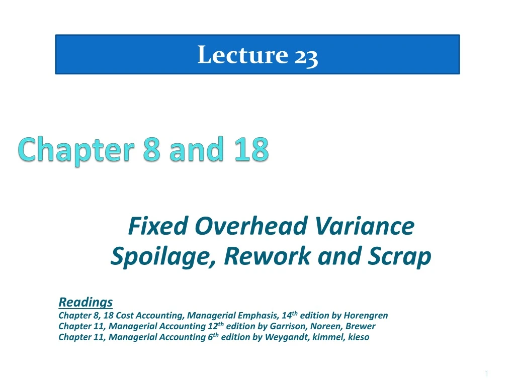
1. Lecture 23 Chapter 8 and 18 Fixed Overhead Variance Spoilage, Rework and Scrap Readings Chapter 8, 18 Cost Accounting, Managerial Emphasis, 14th edition by Horengren Chapter 11, Managerial Accounting 12th edition by Garrison, Noreen, Brewer Chapter 11, Managerial Accounting 6th edition by Weygandt, kimmel, kieso

2. Learning Objectives • Compute the predetermined overhead rate and apply overhead to products in a standard cost system. • Compute and interpret the fixed overhead budget and volume variances. • Accounting for spoilage under different methods of inventory systems and standard costing • Accounting for rework in different situations under different costing methods • Accounting for Scrap in different situations under different costing method • Examples of spoilage

3. Overhead Rates and Overhead Analysis The predetermined overhead ratecan be broken down into fixedand variable components. The variablecomponent is usefulfor preparing and analyzingvariable overheadvariances. The fixedcomponent is usefulfor preparing and analyzingfixed overheadvariances.

4. In a standard costsystem, overhead isapplied to work inprocess based onthe standard hoursallowed for the actualoutput of the period. Normal versus Standard Cost Systems In a normal costsystem, overhead isapplied to work inprocess based onthe actual numberof hours workedin the period.

5. Fixed Overhead Variances Actual Fixed Fixed Fixed Overhead Overhead Overhead Incurred Budget Applied DH × FR SH × FR Budget Variance VolumeVariance FR = Standard Fixed Overhead RateSH = Standard Hours AllowedDH = Denominator Hours

6. Overhead Rates and OverheadAnalysis – Example ColaCo prepared this budget for overhead: Total Variable Total Fixed Machine Variable Overhead Fixed Overhead Hours Overhead Rate Overhead Rate 3,000 $ 6,000 ? $ 9,000 ? 4,000 8,000 ? 9,000 ? Let’s calculate overhead rates. ColaCo applies overhead basedon machine-hour activity.

7. Total Variable Total Fixed Machine Variable Overhead Fixed Overhead Hours Overhead Rate Overhead Rate 3,000 $ 6,000 $ 2.00 $ 9,000 ? 4,000 8,000 2.00 9,000 ? Rate = TotalVariable Overhead ÷ Machine Hours Overhead Rates and OverheadAnalysis – Example ColaCo prepared this budget for overhead: This rate is constant at all levels of activity.

8. Total Variable Total Fixed Machine Variable Overhead Fixed Overhead Hours Overhead Rate Overhead Rate 3,000 $ 6,000 $ 2.00 $ 9,000 $ 3.00 4,000 8,000 2.00 9,000 2.25 Rate = TotalFixedOverhead ÷ Machine Hours Overhead Rates and OverheadAnalysis – Example ColaCo prepared this budget for overhead: This rate decreases when activity increases.

9. Total Variable Total Fixed Machine Variable Overhead Fixed Overhead Hours Overhead Rate Overhead Rate 3,000 $ 6,000 $ 2.00 $ 9,000 $ 3.00 4,000 8,000 2.00 9,000 2.25 The total POHR is the sum ofthe fixed and variable ratesfor a given activity level. Overhead Rates and OverheadAnalysis – Example ColaCo prepared this budget for overhead:

10. Fixed Overhead Variances – Example ColaCo’s actual production required 3,200standard machine hours. Actual fixed overhead was $8,450. The predetermined overhead rate is based on 3,000 machine hours.

11. Overhead Variances Now let’s turn our attention to calculatingfixed overhead variances.

12. Fixed Overhead Variances – Example Actual Fixed Fixed Fixed Overhead Overhead Overhead Incurred Budget Applied $8,450 $9,000 Budget variance$550 favorable

13. Budget Variance Fixed Overhead Variances –A Closer Look Results from spendingmore or less thanexpected for fixedoverhead items. Now, let’s use the standard hours allowed to compute the fixed overhead volume variance.

14. Fixed Overhead Variances – Example Actual Fixed Fixed Fixed Overhead Overhead Overhead Incurred Budget Applied SH × FR 3,200 hours × $3.00 per hour $8,450 $9,000 $9,600 Budget variance$550 favorable Volume variance$600 favorable

15. VolumeVariance Results when standard hoursallowed for actual output differsfrom the denominator activity. Unfavorablewhen standard hours< denominator hours Favorablewhen standard hours> denominator hours Volume Variance – A Closer Look

16. VolumeVariance Does not measure over- or under spending Results when standard hoursallowed for actual output differsfrom the denominator activity. It results from treating fixedoverhead as if it were avariable cost. Unfavorablewhen standard hours< denominator hours Favorablewhen standard hours> denominator hours Volume Variance – A Closer Look

17. Quick Check  Yoder Enterprises’ actual production for the period required 2,100 standard direct labor hours. Actual fixed overhead for the period was $14,800. The budgeted fixed overhead was $14,450. The predetermined fixed overhead rate was $7 per direct labor hour. What was the budget variance? a. $350 U b. $350 F c. $100 F d. $100 U

18. Quick Check  Budget variance = Actual fixed overhead – Budgeted fixed overhead = $14,800 – $14,450 = $350 U Yoder Enterprises’ actual production for the period required 2,100 standard direct labor hours. Actual fixed overhead for the period was $14,800. The budgeted fixed overhead was $14,450. The predetermined fixed overhead rate was $7 per direct labor hour. What was the budget variance? a. $350 U b. $350 F c. $100 F d. $100 U

19. Quick Check  Yoder Enterprises’ actual production for the period required 2,100 standard direct labor hours. Actual fixed overhead for the period was $14,800. The budgeted fixed overhead was $14,450. The predetermined fixed overhead rate was $7 per direct labor hour. What was the volume variance? a. $250 U b. $250 F c. $100 F d. $100 U

20. Quick Check  Volume variance = Budgeted fixed overhead – (SH  FR) = $14,450 – (2,100 hours  $7 per hour) = $14,450 – $14,700 = $250 F Yoder Enterprises’ actual production for the period required 2,100 standard direct labor hours. Actual fixed overhead for the period was $14,800. The budgeted fixed overhead was $14,450. The predetermined fixed overhead rate was $7 per direct labor hour. What was the volume variance? a. $250 U b. $250 F c. $100 F d. $100 U

21. Quick Check Summary Actual Fixed Fixed Fixed Overhead Overhead Overhead Incurred Budget Applied SH × FR 2,100 hours × $7.00 per hour $14,800 $14,450 $14,700 Budget variance$350 unfavorable Volume variance$250 favorable

22. Fixed Overhead Variances –A Graphic Approach Let’s look at a graph showing fixed overhead variances. We will use ColaCo’s numbers from the previous example.

23. Cost $9,000 budgeted fixed OH Fixed overhead applied to products Activity 3,000 Hours ExpectedActivity Fixed Overhead Variances –A Graphic Approach

24. Cost $9,000 budgeted fixed OH Fixed overhead applied to products Activity 3,000 Hours ExpectedActivity Fixed Overhead Variances –A Graphic Approach { $8,450 actual fixed OH $8,450 actual fixed OH $550FavorableBudget Variance

25. Cost $9,000 budgeted fixed OH Fixed overhead applied to products Activity 3,000 Hours ExpectedActivity Fixed Overhead Variances –A Graphic Approach 3,200 machine hours × $3.00 fixed overhead rate $600FavorableVolume Variance $9,600 applied fixed OH { { $8,450 actual fixed OH $8,450 actual fixed OH $550FavorableBudget Variance 3,200 StandardHours

26. Unfavorablevariances are equivalentto underapplied overhead. Favorablevariances are equivalentto overapplied overhead. The sum of the overhead variancesequals the under- or overappliedoverhead cost for a period. Overhead Variances and Under- or Overapplied Overhead Cost In a standardcost system:

27. Closer look at overhead variances The overhead variance is generally analyzed through a price variance and a quantity variance. • Overhead controllable variance(price variance) shows whether overhead costs are effectively controlled. • Overhead volume variance(quantity variance) relates to whether fixed costs were under- or over-applied during the year.

28. Closer look at overhead variances Overhead Controllable Variance The overhead controllable variance shows whether overhead costs are effectively controlled. To compute this variance, the company compares actual overhead costs incurred with budgeted costs for the standard hours allowed. The budgeted costs are determined from a flexible manufacturing overhead budget.

29. Closer look at overhead variances For Xonic the budget formula for manufacturing overhead is variable manufacturing overhead cost of $3 per hour of labor plus fixed manufacturing overhead costs of $4,400.

30. Closer look at overhead variances Overhead Controllable Variance Illustration 11B-2 shows the formula for the overhead controllable variance and the calculation for Xonic, Inc.

31. Closer look at overhead variances Overhead Volume Variance Difference between normal capacity hours and standard hours allowed times the fixed overhead rate.

32. Closer look at overhead variances Illustration:Xonic Inc. budgeted fixed overhead cost for the year of $52,800. At normal capacity, 26,400 standard direct labor hours are required. Xonic produced 1,000 units of Xonic Tonic in June. The standard hours allowed for the 1,000 gallons produced in June is 2,000 (1,000 gallons x 2 hours). For Xonic, standard direct labor hours for June at normal capacity is 2,200 (26,400 annual hours ÷ 12 months). The computation of the overhead volume variance in this case is as follows.

33. Closer look at overhead variances In computing the overhead variances, it is important to remember the following. • Standard hours allowed are used in each of the variances. • Budgeted costs for the controllable variance are derived from the flexible budget. • The controllable variance generally pertains to variable costs. • The volume variance pertains solely to fixed costs.

34. Spoilage, Rework, and Scrap

35. Basic Terminology • Spoilage – units of production, either fully or partially completed, that do not meet the specifications required by customers for good units and that are discarded or sold for reduced prices

36. Basic Terminology • Rework – units of production that do not meet the specifications required by customers but which are subsequently repaired and sold as good finished goods • Scrap – residual material that results from manufacturing a product. Scrap has low total sales value compared with the total sales value of the product

37. Accounting for Spoilage • Accounting for spoilage aims to determine the magnitude of spoilage costs and to distinguish between costs of normal and abnormal spoilage • To manage, control and reduce spoilage costs, they should be highlighted, not simply folded into production costs

38. Types of Spoilage • Normal Spoilage – is spoilage inherent in a particular production process that arises under efficient operating conditions • Management determines the normal spoilage rate • Costs of normal spoilage are typically included as a component of the costs of good units manufactured because good units cannot be made without also making some units that are spoiled

39. Types of Spoilage • Abnormal Spoilage – is spoilage that is not inherent in a particular production process and would not arise under normal operating conditions • Abnormal spoilage is considered avoidable and controllable • Units of abnormal spoilage are calculated and recorded in the Loss from Abnormal Spoilage account, which appears as a separate line item no the income statement

40. Process Costing and Spoilage • Units of Normal Spoilage can be counted or not counted when computing output units (physical or equivalent) in a process costing system • Counting all spoilage is considered preferable

41. Inspection Points and Spoilage • Inspection Point – the stage of the production process at which products are examined to determine whether they are acceptable or unacceptable units. • Spoilage is typically assumed to occur at the stage of completion where inspection takes place

42. The Five-Step Procedure for Process Costing with Spoilage • Step 1: Summarize the flow of Physical Units of Output – identify both normal and abnormal spoilage • Step 2: Compute Output in Terms of Equivalent Units. Spoiled units are included in the computation of output units

43. The Five-Step Procedure for Process Costing with Spoilage • Step 3: Compute Cost per Equivalent Unit • Step 4: Summarize Total Costs to Account For • Step 5: Assign Total Costs to: • Units Completed • Spoiled Units • Units in Ending Work in Process

44. Steps 1 & 2 Illustrated

45. Steps 3, 4 & 5 Illustrated

46. Steps 1 & 2, Illustrated

47. Steps 3, 4 & 5, Illustrated

48. Steps 1 & 2, Illustrated

49. Steps 3, 4 & 5, Illustrated

50. Job Costing and Spoilage • Job costing systems generally distinguish between normal spoilage attributable to a specific job from normal spoilage common to all jobs