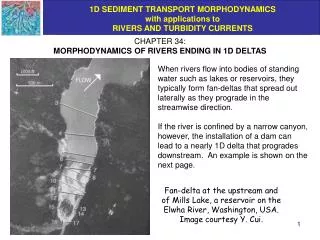
CHAPTER 34: MORPHODYNAMICS OF RIVERS ENDING IN 1D DELTAS

1. CHAPTER 34: MORPHODYNAMICS OF RIVERS ENDING IN 1D DELTAS When rivers flow into bodies of standing water such as lakes or reservoirs, they typically form fan-deltas that spread out laterally as they prograde in the streamwise direction. If the river is confined by a narrow canyon, however, the installation of a dam can lead to a nearly 1D delta that progrades downstream. An example is shown on the next page. Fan-delta at the upstream and of Mills Lake, a reservoir on the Elwha River, Washington, USA. Image courtesy Y. Cui.

2. AN EXAMPLE OF A 1D DELTA Hoover Dam was closed in 1936. Backwater from the dam created Lake Mead. Initially backwater extended well into the Grand Canyon. For much of the history of Lake Mead, the delta at the upstream end has been so confined by the canyon that is has propagated downstream as a 1D delta. As is seen in the image, the delta is now spreading laterally into Lake Mead, forming a 2D fan-delta. View of the Colorado River at the upstream end of Lake Mead. Image from NASA https://zulu.ssc.nasa.gov/mrsid/mrsid.pl

3. HISTORY OF SEDIMENTATION IN LAKE MEAD, 1936 - 1948 Image based on an original from Grover and Howard (1937)

4. STRUCTURE OF A DELTA: TOPSET, FORESET AND BOTTOMSET A typical delta deposit can be divided into a topset, foreset and bottomset. The topset is coarse-grained (sand or sand and gravel), and is emplaced by fluvial deposition. The foreset is also coarse-grained, and is emplaced by avalanching. The bottomset is fine-grained (mud, e.g. silt and clay) and is emplaced by either plunging turbidity currents are rain from sediment-laden surface plumes. standing water

5. SIMPLIFICATION: TOPSET AND FORESET ONLY Here the problem is simplified by considering a topset and foreset only. That is, the effect of the mud is ignored. Mud is included in a later chapter. standing water

6. MOVING BOUNDARIES The problem is charactized by two moving boundaries. The point x = ss(t) corresponds to the topset-foreset break, and the point x = sb(t) corresponds to the foreset-bottomset break. Bed elevation is denoted as (x, t); the antecedent bed profile over which the delta progrades is denoted as base(x). Bed elevation at the topset-foreset break is given as s(t) = [ss(t), t]. Bed elevation at the foreset-bottomset break is given as b(t) = [sb(t), t].

7. EXNER EQUATION OF SEDIMENT CONSERVATION The Exner equation of sediment conservation takes the form An appropriate boundary condition at the upstream end is where qtf denotes a sediment feed rate qtf

8. LINEAR BED PROFILE ON FORESET (DELTA FRONT) Bed elevation on the fluvial region, i.e. 0  x  ss(t) is denoted as f(x,t). The delta front is assumed to have a specified constant angle of avalanching Sa. This angle is usually less, often much less than the angle of repose of the sediment (Kostic and Parker, 20xx). The profile on the foreset is thus given as

9. SHOCK CONDITION ON FORESET (DELTA FRONT) The Exner equation of sediment continuity can be integrated across the delta front to yield the shock condition (Swenson et al., 2000: Kostic and Parker, 2003a,b). Now it is assumed that no (coarse-grained) sediment escapes the toe of the delta front, so that qt[sb(t), t] = 0. In addition, the bed profile across the foreset, can be used to calculate /t across it. Remembering to compute the material derivative of f[ss(t), t], it is found that

10. SHOCK CONDITION ON FORESET (DELTA FRONT) contd. Denoting The condition at the bottom of the last slide reduces to Where Ss denotes the bed slope of the fluvial region at the topset-foreset break. Now substituting the above relation into and integrating, it is found that

11. SHOCK CONDITION ON FORESET (DELTA FRONT) contd. Upon reduction, the shock condition can be reduced to the following form: where qts = qt[ss(t), t] denotes the volume rate per unit width of delivery of bed material load to the brink of the foreset. This condition can be understood in a simple way. Suppose that Ss << Sa and that the term can be neglected. Further noting that the height of the delta front  is equal to Sa (sb – ss), it is seen that the condition reduces to: That is, all the sediment delivered to the topset-foreset break is consumed in prograding the delta forward at speed .

12. CONTINUITY CONDITION AT FORESET-BOTTOMSET BREAK The foreset elevation profile must match continuously with the antecedent bed profile base(x) at the point x = sb(t), i.e. the foreset-bottomset break. Here base is a specified profile. Thus (Kostic and Parker, 2003a,b):

13. CONTINUITY CONDITION AT FORESET-BOTTOMSET BREAK contd. Taking the derivative with respect to time of the equation below yields the result Denoting the basement slope at the foreset-bottomset break as Sb, where the condition reduces to Thus if Ss and Sb are small compared to Sa and the time derivate in f can be neglected, the condition reduces simply to so that the foreset-bottomset break progrades at the same speed as the topset-foreset break.

14. MOVING BOUNDARY FORMULATION The Exner equation on the fluvial zone is transformed using the following moving-boundary coordinates: Note that the fluvial zone is now traversed from sediment feed point to topset-foreset break as . The derivatives transform according to the chain rule as

15. EXNER EQUATION, SHOCK CONDITION AND CONTINUITY CONDITION IN MOVING-BOUNDARY COORDINATES The Exner equation transforms to: The shock condition transforms to: The continuity condition transforms to:

16. IMPLEMENTATION: SEDIMENT TRANSPORT RELATION The calculation is implemented using a generic relation for total bed material transport: where t, nt and c* must be specified. The flow field is computed using a constant Chezy coefficient Cz for simplicity. As was seen in Chapters 19 and 21, the generalization to a) a sediment transport formulation that divides bed material load into bed load and suspended load components, b) a resistance predictor that divides resistance into skin friction and form drag and c) a flow hydrograph is relatively straightforward.

17. IMPLEMENTATION: BACKWATER FORMULATION Deltas are zones where rivers meet standing water. As a result, it can be expected that backwater effects are important in deltas. The backwater formulation was given in Chapter 5. In moving-boundary coordinates, it takes the form with the boundary condition on H of where s denotes the elevation of standing water. Note that the elevation of standing water s can in general be a function of time. It is variation in this parameter that allows the determination of the effect of base level change on delta morphodynamics.

18. IMPLEMENTATION: BACKWATER FORMULATION contd. Once the depth H is computed everywhere at a given time from the backwater formulation, the Shields number * is evaluated from the relation This in turn allows evaluation of qt from the total bed material load equation:

19. IMPLEMENTATION: NORMAL FLOW APPROXIMATION In some cases it is desirable to use the normal flow approximation, even with its disadvantages in the vicinity of a delta. In such case the backwater formulation is replaced with the computation Thus if qw, R, D, Cz and the bed profile  are specified at any time, * and qt can be computed everywhere from the above relations and the load equation; In the backwater formulation, changing base level is mediated by a time-varying elevation of standing water d, where the function must be specified. In a backwater formulation, changing base level is approximated in terms of a time-varying downstream bed elevation. That is, where must be specified. This condition places some limits on the results of the analysis, as outlined in subsequent slides.

20. SPECIFICATION OF THE ANTECEDENT BED PROFILE base(x), THE INITIAL BED CONFIGURATION AND THE UPSTREAM BOUNDARY CONDITION Although in general the antecedent bed profile can be specified arbitrarily, here it is assumed for simplicity that this profile has constant bed slope - base/x = Sbase. The upstream end of the fluvial zone is always located at x = 0. The initial length of the fluvial zone is ssI and the initial bed slope is SfI. The initial elevation of the topset-foreset break is sI, and the initial elevation of the bottom of the topset-foreset break is bI. The initial bed profile is thus given as The antecedent bed profile is a straight line with slope Sbase and passing though elevation bI at x = ssI + (sI - bI)/Sa. In any calculation, Sb, ssI, SfI, sI, bI and foreset slope Sa must be specified by the user. The upstream boundary condition is specified in terms of a sediment feed rate qtf, which in general may vary in time.

21. FLOW OF THE CALCULATION: BACKWATER FORMULATION • For any given time : • Specify the elevation of downstream standing water d. • Calculate the backwater curve upstream from . • Use this to evaluate qt everywhere, including qts at . • Implement the shock condition to find . This shock condition requires knowledge of the term • It is sufficient to evaluate this term using the current bed profile and that obtained one step earlier. At this term can be ignored. • Solve Exner everywhere to find new bed elevations at time later. • Use continuity condition to find . • Update boundaries:

22. FLOW OF THE CALCULATION: NORMAL FLOW FORMULATION • For any given time : • Specify the downstream bed elevation d. • Calculate the bed slope S everywhere, and use this to find H everywhere. • Use this to evaluate qt everywhere, including qts at . • Implement the shock condition to find . This shock condition requires knowledge of the term • This term can be directly computed in terms of the imposed function . • Solve Exner everywhere except the last node (where bed elevation is specified) to find new bed elevations at time later. • Use continuity condition to find . • Update boundaries:

23. DISCRETIZATION AND SPECIFICATION OF INITIAL BED Initial bed

24. CALCULATION OF DERIVATIVES Two Excel workbooks with code are presented here. The backwater formulation is given in RTe-book1DDeltaBW.xls, and the normal flow formulation is given in Rte-book1DDeltaNorm.xls. In both cases the spatial derivative of f appearing in the transformed Exner relation is computed using a central difference scheme except at end nodes. That is, In the case of the normal flow formulation, it is not necessary to compute the above derivate at node M + 1, because bed elevation d is specified there.

25. CALCULATION OF DERIVATIVES contd. Spatial derivatives in qt should be based on an upwinding scheme for a backwater formulation. In the code presented here, a pure upwinding scheme is used for all nodes, i.e. A partial upwinding scheme will also work. In the case of a normal flow formulation, spatial derivatives in qt can be based on a central difference scheme for internal nodes: Again, in the normal flow formulation the above derivative need not be computed at node M = 1.

26. INTRODUCTION TO Rte-book1DDeltaBW.xls The code in this spreadsheet uses a backwater formulation. Input variables include Flood discharge/width qw Time step t Flood intermittency If No. of spatial intervals M Chezy resistance coefficient Cz Steps to printout Mtoprint Grain size D Printouts beyond initial Mprint Sed submerged specific gravity R Deposit porosity lp Volume bed material feed rate/width qtf Coefficient in bed material transport relation at Exponent in bed material transport relation nt Critical Shields number in transport relation c* Elevation of downstream standing water d Initial elevation of topset-foreset break sI Initial elevation of foreset-bottomset break bI Initial bed slope of fluvial zone SfI Bed slope of subaqueous basement Sb Initial length of fluvial zone sfI Maximum length of fluvial zone sfmax Slope of avalanching on foreset Sa The code uses a fixed elevation d of standing water at the downstream end. The code can be easily modified to handle the case of time-varying base level.

27. CALCULATIONS WITH Rte-book1DDeltaBW.xls Calculations are presented for the indicated input parameters, except for Mtoprint, which is varied to capture the time evolution of the river profile.

28. Note how the backwater formulation captures the new delta front as it progrades over the antecedent bed. Mtoprint = 20

29. Mtoprint = 100

30. The incipient delta merges with the antecedent one, which then progrades outward vigorously. Mtoprint = 200

31. Progradation with a nice upward-concave long profile. Mtoprint = 5000

32. The calculation craps out for Mtoprint = 10000 (final time = 30 years).

33. Not to worry. Just increase the number of spatial intervals M from 20 to 40 and it works fine for Mtoprint = 10000 (final time = 30 years)!

34. The conditions for this run are identical to those of the previous slide, except that basement slope Sb has been changed from 0 to 0.0003. Note that the long profiles are less concave, and that the progradation rate is reduced.

35. WORKSHEET InData OF Rte-book1DDeltaBW.xls PROVIDES USEFUL GUIDANCE IN REGARD TO INPUT PARAMETERS • Make sure that d > sI! • If initial depth Hi = d - sI is less than Hcrit then the flow will be locally supercritical and the calculation will fail! • If Hi < Hni, where Hni = normal depth for the initial bed, then the initial flow will follow an M2 curve, which requires a very dense spatial grid to capture. • Certain combinations of sI, bI and d will cause the calculation to fail as the height of the foreset falls to zero. Increasing sI usually fixes the problem. • As always, it is necessary to tinker with t and M to obtain numerical stability.

36. AN EXAMPLE OF A CALCULATION FAILURE All parameters are the same as those of slides 27 and 31 except that d has been lowered from 8.5 m to 7 m. The calculation fails for the very physical reason that the delta front is prograded out of existence. To get the calculation to work, either raise d or lower bI.

37. EXAMPLE OF A HIGH BASE LEVEL This case is the same as that of slide 30 (Mtoprint = 200), except that d is increased from 8.5 m to 20 m. Note how this retards delta progradation.

38. INTRODUCTION TO Rte-book1DDeltaNorm.xls The code in this spreadsheet uses a normal flow formulation. Input variables include Flood discharge/width qw Time step t Flood intermittency If No. of spatial intervals M Chezy resistance coefficient Cz Steps to printout Mtoprint Grain size D Printouts beyond initial Mprint Sed submerged specific gravity R Deposit porosity lp Volume bed material feed rate/width qtf Coefficient in bed material transport relation at Exponent in bed material transport relation nt Critical Shields number in transport relation c* Elevation of topset-foreset break d Initial elevation of foreset-bottomset break bI Initial bed slope of fluvial zone SfI Bed slope of subaqueous basement Sb Initial length of fluvial zone sfI Slope of avalanching on foreset Sa The code uses a fixed bed elevation d at the downstream end. The code can be easily modified to handle the case of time-varying base level, but if d rises too rapidly in time the delta goes into autoretreat, requiring special treatment. See Chapter 38.

39. CALCULATIONS WITH Rte-book1DDeltaNorm.xls The input conditions are identical to slide 27 (backwater formulation), except that base level is specified in terms of a fixed downstream bed level d. Calculations are presented for the indicated input parameters, except for Mtoprint, which is varied to capture the time evolution of the river profile.

40. This case (normal flow) corresponds to slide 31 (backwater). By this time the results are not much different between the two.

41. The two cases (backwater versus normal) are compared at the end time (15 years) of slides 31 and 40. The profile for the backwater calculation has prograded less, because the specified downstream water surface elevation of 8.5 m has led to a computed downstream bed elevation that is higher than the specified value of 3 m for the normal flow calculation.

42. This case (normal flow) corresponds to slide 29 (backwater). At this earlier time, the difference between the two is fairly strong.

43. In the case of the backwater calculation, the antecedent delta is still inactive by 0.3 years as the deposit struggles to overcome backwater upstream. In the case of the normal flow calculation, the antecedent delta is forced to prograde immediately, as there is no backwater.

44. NOTES IN CLOSING •  This formulation uses a constant Chezy resistance coefficient. • Could you modify it for Manning-Strickler? For Wright-Parker? • This formulation uses a relation for total bed material load  Could you modify it to treat bed load and suspended load separately?  This formulation assumes a uniform sediment size Could you modify it to treat sediment mixtures?  This formulation assumes constant base level at the downstream end. Could you modify it to treat time-varying base level?  This formulation assumes an intermittency and a constant flood flow. Could you modify it to treat hydrographs? The purpose of this e-book is not to work out each one of these permutations. Rather the purpose is to provide the reader with the necessary tools to allow adaptation to specific research and engineering problems of interest.

45. REFERENCES FOR CHAPTER 34 Grover, N.C., and Howard, C.L., 1937, The passage of turbid water through Lake Mead, Transactions, American Society of Civil Engineers, 103, 720-732. Kostic, S. and Parker, G., 2003a, Progradational sand-mud deltas in lakes and reservoirs. Part 1. Theory and numerical modeling, Journal of Hydraulic Research, 41(2), 127-140. Kostic, S. and Parker, G., 2003b, Progradational sand-mud deltas in lakes and reservoirs. Part 2. Experiment and numerical simulation, Journal of Hydraulic Research, 41(2), 141-152 Swenson, J. B., Voller, V. R., Paola, C., Parker G. and Marr J., 2000, Fluvio-deltaic sedimentation: a generalized Stefan problem, European Journal of Applied Math., 11, 433-452.