Forecasting
Forecasting. The future is made of the same stuff as the present. – Simone Weil. Demand Forecast. Resource Planning. Aggregate Production Planning. Rough-cut Capacity Planning. Master Production Scheduling. Bills of Material. Material Requirements Planning. Inventory Status. Job

Forecasting
E N D
Presentation Transcript
Forecasting The future is made of the same stuff as the present. – Simone Weil
Demand Forecast Resource Planning Aggregate Production Planning Rough-cut Capacity Planning Master Production Scheduling Bills of Material Material Requirements Planning Inventory Status Job Pool Capacity Requirements Planning Job Release Routing Data Job Dispatching MRP II Planning Hierarchy
Forecasting • Basic Problem: predict demand for planning purposes. • Laws of Forecasting: 1. Forecasts are always wrong! 2. Forecasts always change! 3. The further into the future, the less reliable the forecast will be! • Forecasting Tools: • Qualitative: • Delphi • Analogies • Many others • Quantitative: • Causal models (e.g., regression models) • Time series models
Forecasting “Laws” 1) Forecasts are always wrong! 2) Forecasts always change! 3) The further into the future, the less reliable the forecast! 40% Trumpet of Doom 20% +10% -10% Start of season 16 weeks 26 weeks
Quantitative Forecasting • Goals: • Predict future from past • Smooth out “noise” • Standardize forecasting procedure • Methodologies: • Causal Forecasting: • regression analysis • other approaches • Time Series Forecasting: • moving average • exponential smoothing • regression analysis • seasonal models • many others
Time Series Forecasting Historical Data Forecast Time series model f(t+t), t = 1, 2, … A(i), i = 1, … , t
Time Series Approach • Notation:
Time Series Approach (cont.) • Procedure: 1. Select model that computes f(t+t) from A(i), i = 1, … , t 2. Forecast existing data and evaluate quality of fit by using: 3. Stop if fit is acceptable. Otherwise, adjust model constants and go to (2) or reject model and go to (1).
Moving Average • Assumptions: • No trend • Equal weight to last m observations • Model:
Moving Average (cont.) • Example: Moving Average with m = 3 and m = 5. Note: bigger m makes forecast more stable, but less responsive.
Exponential Smoothing • Assumptions: • No trend • Exponentially declining weight given to past observations • Model:
Exponential Smoothing (cont.) • Example: Exponential Smoothing with a = 0.2 and a = 0.6. Note: we are still lagging behind actual values.
Exponential Smoothing with a Trend • Assumptions: • Linear trend • Exponentially declining weights to past observations/trends • Model: Note: these calculations are easy, but there is some “art” in choosing F(0) and T(0) to start the time series.
Exponential Smoothing with a Trend (cont.) • Example: Exponential Smoothing with Trend, a = 0.2, b = 0.5. Note: we start with trend equal to difference between first two demands.
Exponential Smoothing with a Trend (cont.) • Example: Exponential Smoothing with Trend, a = 0.2, b = 0.5. Note: we start with trend equal to zero.
Effects of Altering Smoothing Constants • Exponential Smoothing with Trend: various values of a and b Note: these assume we start with trend equal diff between first two demands.
Effects of Altering Smoothing Constants • Exponential Smoothing with Trend: various values of a and b Note: these assume we start with trend equal to zero.
Effects of Altering Smoothing Constants (cont.) • Observations: assuming we start with zero trend • a = 0.3, b = 0.5 work well for MAD and MSD • a = 0.6, b = 0.6 work better for BIAS • Our original choice of a = 0.2, b = 0.5 had MAD = 3.73, MSD = 22.32, BIAS = -2.02, which is pretty good, • although a = 0.3, b = 0.6, with MAD = 3.65, MSD=21.78, BIAS = -1.52 is better.
Winters Method for Seasonal Series • Seasonal series:a series that has a pattern that repeats every N periods for some value of N (which is at least 3). • Seasonal factors:a set of multipliers ct, representing the average amount that the demand in the tth period of the season is above or below the overall average. • Winter’s Method: • The series: • The trend: • The seasonal factors: • The forecast:
Winters Method - Sample Calculations • Initially we set: • smoothed estimate = first season average • smoothed trend = zero (T(N)=T(12) = 0) • seasonality factor = ratio of actual to • average demand From period 13 on we can use initial values and standard formulas...
Conclusions • Sensitivity: Lower values of m or higher values of a will make moving average and exponential smoothing models (without trend) more sensitive to data changes (and hence less stable). • Trends: Models without a trend will underestimate observations in time series with an increasing trend and overestimate observations in time series with a decreasing trend. • Smoothing Constants: Choosing smoothing constants is an art; the best we can do is choose constants that fit past data reasonably well. • Seasonality: Methods exist for fitting time series with seasonal behavior (e.g., Winters method), but require more past data to fit than the simpler models. • Judgement: No time series model can anticipate structural changes not signaled by past observations; these require judicious overriding of the model by the user.