Modeling Biological Systems Goals
470 likes | 843 Vues
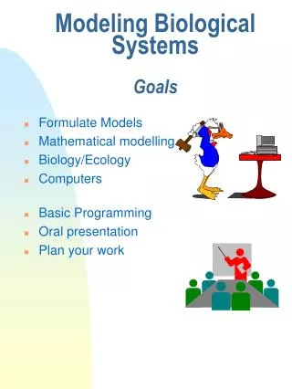
Modeling Biological Systems Goals. Formulate Models Mathematical modelling Biology/Ecology Computers Basic Programming Oral presentation Plan your work. Course Outline. Lecture Work on project Oral presenation of project New chapter. Uno Wennergren

Modeling Biological Systems Goals
E N D
Presentation Transcript
ModelingBiological SystemsGoals • FormulateModels • Mathematicalmodelling • Biology/Ecology • Computers • Basic Programming • Oral presentation • Plan your work
CourseOutline • Lecture • Work on project • Oral presenation of project • New chapter
Uno Wennergren Professor Theoretical Biology • OrganicFarming • Threatened Species • Spread of disease • Animal Welfare • 6 PhD students5 senior researchers
SubjectsChapters in the book • Basic about models • Discrete Processes • Deterministic models • Stochastic models • Continous processes • Deterministic models • (Stochastic models –excluded)
Methods/Tools • Graphic methods - Cobweb • Spreadsheets - Excel • Programing - Matlab • Mathematical Analysis
Methods/Tools • Planning • PowerPoint • Excel • Oral presentations Computer-OH projector
Project • Plan your time, time schedule • Formulate the problem • Choose • Type of mathematicalmodel • Whatmethods and tools to use • How to present the results • Re-plan • Construct the model • Ifpossibleusecritical test • Implement the model by excel or matlab • Re test the model • Ifpossibleusecritical test • Make the code and a ppt presentation tidy – presentable to Uno, Stefan and Peter • For whom it mayconcern: prepare for oral presentation. This yeareverytime!
Basic about Models • A model is a description of reality • A mathematical model uses equations to describe reality • Two levels of modeling Dn/dt=rn(t) I Simplified Reality II Mathematical equations Complex reality
Basic about Models • A modelusually has a purpose • The questions: • Is the realitysimplifiedenough to be represented by equations? • Is the realitysimplifiedtoomuch and hence the model is no longer a description of reality (not useful)? Dn/dt=rn(t) I Simplified Reality II Mathematical equations Complex reality Test thesequestions in your projects
Discrete Dynamical Systems • Discrete processes • Events stepwise • perennialsreproduction (seeds) 1 time/year • Continous processes • Events all the time • Small mammmalsreproduction year around • Perennials survival? • insects reproduction? • in temperate climates?
Deterministic models • Models don’t include variation/chance probability. Parameters are constant • All process are the same (within a specific model) and simply a specific chain of events. • The result is deterministic: one value • Stochastic models include variation/chance probability • The result is a set of values • Every test generates a new chain of events with its specific result
Recurrenceequations(Markovchain) • The equation generates a sequence of numbers • The equation calculates a number by using some of the previous number.Example: How many were infected previously determines how many will be infected right now. Which in its turn….. • Note: specific step lengths
Recurrence equations(linear) • General formx(n)=f(x(n-1),x(n-2),….) • The order of the equation is set by the number of steps backwards used in the equation x(n)=7x(n-5)is of order 5. • How many initial values (numbers) do you need to start the equation to roll? • Assume simple growth:x(n+1)=Rx(n)
Model type:Difference equaions(number sequence) • Of first order: f(x(n-1)) =x(n)-x(n-1) • Compare with differential The derivative of f(x): Rearrangerecurrenceeq:
Box diagram • Simple growth • x(n)-x(n-1)=rx(n-1) • x(n+1)=x(n)(1+r) rx Population x growth bx Population x (1-s)x deaths fecundity i immigration
Mathematical analysis • Simplest linear recursive equationx(n+1)=Rx(n)has the solution • x(n)=Rnx(0)growths exponentially: R>1decrease exponentially:0<R<1OscillatesR<-1constant or oscillates if R0,1,-1 • What about -1<R<0???
Spreadsheets • Click and drag • Relative addresses • =C1*B4 • absolute adresses • =$C1*B5 • =$C$1*B5
Matematical analysis • Equlibrium points • Will the sequence stop at a point? Comes back to itself. • Is it stable or unstable?Compare with valley and hilltop. • Find and calculate the equlibrium point: • Assume is the equlibrium point test in your equation for example x(n+1)=Rx(n) +aset all for big nThen
Matematical analysis • Equlibrium points • x(n+1)=Rx(n) +agivesNote initial value doesn’t effect whre the equlibrium is • The quilibriumpoint is stable if and only if Compare with xn=f(xn-1)
Cobweb Diagram • Graphic method to find the equlibrium points y y=x Stable equlibrium y=f(x) x y=f(x) is a discrete linear model For examplex(n+1)=-0.5x(n)+4 can be written as y=-0.5x+4
Cobweb diagram • Initial value x* • Next step is y=f(x) y y=x y=f(x) x* x
Cobweb diagram • Next step to take is x=y y y=x y=f(x) x* x
Cobweb diagram • And then y=f(x) y y=x y=f(x) x* x
Cobweb diagram • And then this proceeeds, next step is: x=y y y=x y=f(x) x* x
Cobweb diagram • And y becomes y=f(x) y y=x y=f(x) x* x Just proceed and the curve will stepwise move towards the equilibrium if it’s a stable one
Cobweb diagram • If it steps away from the equlibrium then it’s an unstable one. y y=f(x) y=x x* x
Linear recurrence equation with constant coefficients • Look for a solution, compare withx(n)=Rnx(0) • A linear combination of x(i) terms, for example m number of terms:This is a homogeneous equation since the right hand side is 0. The simplest linear homogenous equation is: ax=0 • How to solve it? • Calculate the roots to the characteristic equation • Matlab funktion r = roots(c)
Characteristic equation • Assume the solution:after some calculations: • This is the charactersitisc equation, use Matlab funktion r = roots(c)
Characteristic equation • Use Matlab funktion r = roots(c) • Or just try it yourself without compuer….. • for x(n)-2x(n-1)+x(n-2)=0 • The charac equation becomes» r=roots([1 -2 -1])r =2.4142 -0.4142
Charactersitic equation • Roots to x(n)-2x(n-1)+x(n-2)=0» r=roots([1 -2 -1])r =2.4142 -0.4142 • General solution isx(n)=C12.4142n - C20.4142n • Particular solutions, we know that x(0)=0 and x(1)=1 gives that • C1+C2=0 which we can use in • 1= C12.4142 - C20.4142 • C1=1/2, C2=-1/2
Charactersitic equation • Roots of x(n)-2x(n-1)+x(n-2)=0 x(n)=C12.4142n - C20.4142nC1=1/2, C2=-1/2gives particular solution • x(n)=1/2(2.4142n - 0.4142n)for big n the first tem dominates (large absolute value)hence: x(n)1/2(2.4142n)
Finite limited growth • Simple assumptions Simplifiedreality • When population is zero there is no reduction in individual growth, no competition, i. e. max growth R • When population is at a equlibrium it has reached its limits and use the resources, K, such that mean individual growth is zero. Hence: The curve of individual growth in relation to density shall pass the points: (0,R),(K,0)
Finite limited growth The curve of individual growth in relation to density shall pass the points: (0,R),(K,0) growth r(x) R population x K Linear model:
Logistic growth R Growth r(x) population x K Linear model: Since x(n)-x(n-1)=r(x(n-1))x(n-1) Or even better x(n+1)=x(n)(r(x(n))+1) with r(x) as above we then have
At right handside there is a quadratic term, x(n),, this is a nonlinear equation! To calculate the equilibrium: Once again assume that there is a equilibrium: Then this have to be true This is a second degree equation with roots: Determine the character of the eq. points:: Test:
If individual maximum (unlimited) growth, R, is larger or qual to 2 there is no stable eq. and chaos and oscillations will appear.
Host parasite model • Assumptions, simplified reality: The host population N growths according to limited logistic growthAdd a term that represent how survival decease as the number of parasites, P, increase
Host parasite model • Host population equaion • The growth of the parasite population also depend on the probability that a host and parasite meet: Assuming proportional to these occasions:
Host parasite model • System of non linear difference equationsLook for equlibriumsSolution (N,P): • (K,0) • (1/Q,R/C(1-1/(QK))) • (0,0)
CourseOutline • Lecture (+ read the chapter, Monday) • Work on project (Tuesday-Thursday) • Oral presenation of project (Friday) • New chapter (Monday) • Faster…….. Projects: Choose between 1.2, 1.3, 1.4, 1.6, 1.8 And if you choose 1.7 you may have to adjust/add something. Discuss with teachers. (Thursday) Uno Wennergren Stefan Sellman Peter Brommesson
Kunskapstaxonomi fritt efter Benjamin Bloom • Fakta. Ange, räkna upp fakta, definiera begrepp. • Enkel begränsad kunskap. • Beskrivning. Innebörden av begrepp och fakta. Tolka, motivera, relatera till varandra. • Tillämpning. Vad är innehållet användbart till. Observera, beräkna, kalkylera, formulera, konstruera, lösa givna problem. • Analys. Bryta ner innehållet, dela upp, gruppera om, jämföra, generalisera se nya problem. • Syntes. Dra slutsatser, formulera regler, se samband också med annan kunskap, resonera, diskutera, skapa nytt. • Värdering. Avge omdömen, kritisera, värdera olika kunskap, hypoteser och teorier mot varandra. • Komplex, vidsträckt kunskap.