QueueTraffic and queuing theory
QueueTraffic and queuing theory. +. Queues in everyday life. You have certainly been in a queue somewhere. Where? How were they different?. At ticket vending machines, cash desks, at the doctors, at printers, in a call center, …. We encounter queues all the time!.

QueueTraffic and queuing theory
E N D
Presentation Transcript
Queues in everyday life You have certainly been in a queue somewhere. • Where? • How were they different? At ticket vending machines, cash desks, at the doctors, at printers, in a call center, … We encounter queues all the time!
Examples: supermarket, doctor • Supermarket: many cash desks,many queues • They even might have an expressqueue line! • Doctor: one doctors (~cash desk),one queue • Similar: queues in a self service restaurant, queues in front of a cable car
What is it about today? • Learn a mathematical model • How are queues analyzed? • What are important concepts and terms for this? Learning goals with the use of QueueTraffic • Being able to explain the concepts arrival rate, throughput, utilization and calculate those for given situations with the help of QueueTraffic • Being able to interpret different values for utilization: Do we get a queue or not? • Being able to explain the difference between Poisson and uniform distribution in a illustrative way
The best system? What is better, what worse? • Many cash desks? • Fast lines? • Number tickets? • ...? • Cannot be decided like this! • What can be decided: How well works a system in a certain situation.
Waiting queues and me:2 points of view • I am responsible for the setting of queues • Manager of a store • Doctor in a medical practice • Operator of a cable car • ... • I am waiting in a queue • Client • Patient • Hiker • ... I can control the system I am depending on the system
Problems of a store manger • When and why do we get queues? • What can we do about it? • Too many people, too few desks • More cash desks • What if there are too many desks open? • Let on more people in • First serve the people who need little service time • Limit the time during which someone is being served costs, boredom, … e.g. printers that sorts job by their size e.g. limited treatment time per client at the doctor
Problems of a customer • Why does it always feel to us like all other queues move faster? • Which queue should I take? Where shall I append? How long do I have to wait? • Where there are the fewest people in queue? • Where the people have the least products to dispatch? • Where the fastest cashier is? • Where one can only pay cash? • Where someone helps me bagging? • ...?
We observe From the left he queue gets extended From the right the queue gets shortened
Arrival and service-process The act of new clients permanently putting theirselves in queue is called arrival process. The number of clients adding theirselves to the queue within a certain period of time is called the arrival rate λ. The act of clients being cleared from queue from the right is called service process. The time one service process takes for one client is called the service time b.
Arrival rate λ (lambda)und service time b • Arrival rate λ: How often do new clients arrive? • Service time b: how long takes a service station for one client? • In a supermarket 5 clients come through the door per hour, on average. Arrival rate: λ = 5/60 clients/minute • It take the man at the cashier on average 15 minutes to serve a client. service time: b = 15 minutes/client
throughput μ (Mu) Throughput μ: How many clients are served per time unit? The throughput is the reciprocal of the service time: μ = 1/b Example: service time b = 15 minute/client Throughput: μ = 1 / 15 clients/minute= 1 client / 15 minutes = 4 clients/hour
Utilization (Rho) Utilization = λ/μ:How much of the capacity of the system is used? Important parameter for the analysis of queuing systems! 3 examples: • λ1 = 10 clients/hour, μ1 = 30 c./h • λ2 = 30 c./h, μ2 = 30 c./h • λ3 = 60 c./h, μ3 = 30 c./h Utilization: 1 =1/μ1 = 10 / 30 = 0.33 2 =2/μ2 = 30 / 30 = 1 3 =3/μ3 = 60 / 30 = 2
Distributions at the arrival Arrivals in QueueTraffic are uniform or Poisson distributed. or
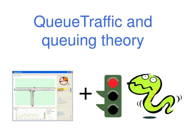
QueueTraffic: Demo Source: http://swisseduc.ch/compscience/infotraffic/
QueueTraffic • Situation and help • Simulation area • Traffic control • Volume of traffic • Simulation control • Data and charts
You solve some first exercises Solve exercises A until 3.
Theoretical and effectivethroughput in in QueueTraffic • So far, we only considered the theoretical throughput μt, since we took at look at how many clients (cars) can be served (drive through) under optimal conditions. • QueueTraffic is a simulation and to calculate the throughput it counts the number of cars driving over the crossroad per round. This is called the effective throughputμe.
Why do we need theeffective throughput? • Fact: How many car could theoretically get through cannot easily be measured or counted. • The number of “served” cars can easily be counted! • This gives us the effective throughput μe • μe = μt is reached, if > μt, i.e. if “enough” cars arrive.
Sample - calculation • Arrival rate: • = 10 car/60s • Effective throughput: • e = 10 cars/60s • Theoretical throughput: • t = (28 s/60s) * (1 car/1s) = 28 cars/60s • Utilization: • = / t= (10 cars/60 s) / (28 cars/60 s) = 0.36 !!! simulated!(counted) calculated!
Remarks to the calculationsin QueueTraffic • Traffic volume is per 60 s • Formula for theoretical throughputμt = „proportion green time” * capacity per lane e.g.: μt = 28s/60s * 1 car/s • Use the theoretical throughput μt to calculate the utilization: = / t given!
The most important terms term example Arrival rate λ 12 cars/minute Service time b 0.1 minute/car throughput t = 1/b 10 cars/minute utilization = / t 1.2
Connection between utilization = / t and traffic jam. In general holds: • < 1 no (or little) jam: system under-worked • ≈ 1 „a little“ jam: system loaded • > 1 growing jam: system overloaded Practical Interpretation: Jam if >t, i.e. if the arrival rate is bigger than the (theoretical) throughput. • Thus: If more cars arrive than what can be served, we get jam!
What was it about today? • Get to know a mathematical model • How are waiting queues analyzed? • What are important terms and concepts? Concrete goals: • Being able to explain the concepts arrival rate, throughput, utilization and calculate those for given situations with the help of QueueTraffic • Being able to interpret different values for utilization: Do we get a queue or not? • Being able to explain the difference between Poisson and uniform distribution in a illustrative way
THE END QueueTraffic undqueuing theory Remarks andfeedback please to: rarnold@wherever.ch http://swisseduc.ch/informatik/infotraffic/

