CHAPTER SEVEN Groundwater
CHAPTER SEVEN Groundwater. Engineering Hydrology (ECIV 4323). Instructors: Dr. Yunes Mogheir Dr. Ramadan Al Khatib. 1. The occurrence of groundwater. Aquifer: the water bearing strata Unconsolidated formation: sands, gravel (Porous aquifer)

CHAPTER SEVEN Groundwater
E N D
Presentation Transcript
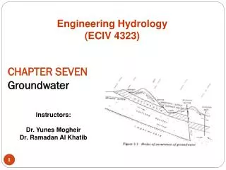
CHAPTER SEVENGroundwater Engineering Hydrology (ECIV 4323) Instructors: Dr. Yunes Mogheir Dr. Ramadan Al Khatib
1. The occurrence of groundwater • Aquifer: the water bearing strata • Unconsolidated formation: sands, gravel (Porous aquifer) • Consolidated formation: sandstone, limestone (karstic aquifer) • Permeability: the measurement of resistance of underground flow due to gradational forces.
Type of aquifer • Confined aquifer • Unconfined aquifer • Phreatic surface, spring, impermeable, river, confined, artesian spring, artesian well, fault
5.2 Factors of Influence • Groundwater flow is laminar. • Density: greater importance is salinity • Viscosity: measure of shear strength of a liquid
5.2 Factors of Influence • Porosity: • (Ranges from few% to 90%) • The more regular the soil, the more porous it tends to be. • Effective porosity ne • In coarse gravel’s ne = n, • in fine material the difference may be 5%,
5.2 Factors of influence • Permeability: is a function of • Porosity, • Structure (grain size, shape of the particles, distribution), • Geological history • Permeability may vary in horizontal and vertical directions (anisotropic) • Permeability is defined by permeability coefficient (k) • For homogeneous rounded grain media: k (m/d) = c (d10 )2 • d10 = the grain size in mm where 10% is finer and 90% is coarse • c: constant 400-1200 • This formula is widely used with sand filter for water supply. It only applies to homogeneous rounded grain media.
k for clean gravel 1-100 cm/s, fine sand 0.001-0.05 cm/s, Clay <10-6 cm/s
5.3 Ground flow • Darcy law: applied under the following assumption: • The material is homogenous and isotropic • There is no capillary zone • Steady state of flow • v = rate of flow/unit area • which is proportional to i, • where i = gradient of potential head
5.3 Ground flow • Note that the specific velocity used in Darcy’s law is not the actual velocity; but is merely Q/A • The actual velocity in the pores is greater than the specific velocity (why?).
5.3.1 Flow in a confined aquifer If there is no change in flow from point to point: Then,
5.3.1 Flow in phreatic aquifer (unconfined) • Darcy law: • vs =-k dφ/dL • By using Dupuit assumptions • Then dφ/dL = dh/dx
5.3.1 Flow in phreatic aquifer (unconfined) • The following is a proof of how
5.3.1 Flow in Phreatic Aquifer (unconfined) • The case of having Net Infiltration N from rainfall
5.4 The abstraction of groundwater • Steps for well drilling • Rotary method is commonly used • As the well drilled it is cased with steel casing to prevent wall collapse • Screen is constructed at the bottom of the well • The screen is covered by gravel packs • Once the water has entered though the well it has to be pumped to the surface by pumps (rotating vertical shaft; submersible)
5.4 The abstraction of groundwater • PVC pipes and screens are available from • 33mm diameter to 630mm diameter
5.5 The yield of well • 5.5.1 Steady confined flow • Darcy law: Q=A vs =-k ds/dr . 2πrH • Q=Q0 ………..continuity
5.5 The yield of well • 5.5.1 Steady confined flow • Darcy law: Q=A vs =-k ds/dr . 2πrH • Q=Q0 ………..continuity Theim’s equation: S1-S2=(Q0/2 πkH )x ln(r2/r1) (KH is transmissibility coefficient ) Valid for steady and unsteady, confined and unconfined
5.5 The yield of well • S= (Q0/2 πkH) x ln(r)+c • S=0 when r=R • S= (Q0/2 πkH) x ln(R/r) • Q0&R can be determined from the boundary conditions • Q0: constant discharge of the well • R=R0 where the drawdown is close to the well that is important
5.5 The yield of well • 5.5.2 Steady unconfined flow • When the drawdown is slight comparing with H use the case of confined aquifer • Darcy flow: • Q=2πr.h.k.(dh/dr) • Q=Q0
5.5 The yield of well 5.5.2 Steady unconfined flow h2=Q0/πk . ln(r) +c if h = H, at r = R H2-h2 = Q0/πk . ln(R/r) (boundary conditions) Well face (H-h0) -- H2-h02 = Q0/πk . ln(R/r0)
5.5 The yield of well 5.5.2 Steady unconfined flow with rainfall Q=2 πr.h.k.(dh/dr) For continuity dQ=-2πr.dr.N (N=net infiltration) Q= -πr2N+C Q= -πr2N+Q0 where r =r0=0, Q=Q0
5.5 The yield of well h2=Q0/πk . ln(r) +Nr2/2k+C2 r=R h=H S=H2- Q0/πk . ln(R)+N/2k . R2 (depend on boundary conditions) H2-h2 = Q0/πk x ln(R/r) – N/2k . (R2-r2) When Q0 = 0 (No pumping) H2-h2 =– N/2k . (R2-r2)
5.6 Test Pumping Analysis • In addition to boring test which provide information about the geology of the aquifer, the extent of the yield aquifer can finally be determined only by pumping test. • Pumping test: • The extent of the yield of an aquifer can finally be determined only by test pumping from a well. • Such a well should be positioned so that observation wells are placed on either side of it, on a line through the well, and preferably on two lines at right angles with the pumping well at the intersection. • Pumping tests can be performed by pumping from the well until steady-state conditions are obtained. • Observation wells should be placed at increasing intervals from the pumping well (say at 20, 50, 100, 200, and 500 m)
5.6 Test Pumping Analysis • Pumping test in confined aquifer • S= Q0/2πkH x ln(R/r) • Observed S are plotted against • distance r (logarithmic scale) • then straight line is obtained where • S=A-Blog(r) • Then • kH=(1/B) . (1.15Q0/π)
…example 5.5 First, draw the relationship between s and log(r). The graph is shown in the previous slide. This will give you a linear relationship. The slope of the resulting line is B. The resulting line will intersect the x-axis at the radius of influence ( since s = 0). To compute B: at s = 0, r = 610 and log(r) = 2.79 at s = 1.2, r = 10 and log(r) = 1.0 B = (1.2 – 0)/(2.79 – 1.0) = 0.67 , which is the slope of the line kH = (1/B) . (1.15Q0/π) = (1/0.67).(1.15) . (0.03 / π) = 1.64x10⁻² m2/s To find the radius of influence, R: The line intersects the x-axis at the value of R (since this is corresponding to a zero drawdown). → R = 610 m To find the value of A: slope = 0.67 = y/x = A / log(610) A = (0.67) . Log(610) = 2.79