Download
1 / 18
240 likes | 767 Vues
Turing Machines as Transducers. Turing-computable Functions. Function f with domain D is computable if There exists TM M= (Q, D, , , q 0 , B , F) Such that for all w D q 0 w ├* q f f(w) for some q f F. Create TMs for the following. f(w) = cwc (w {0,1}*)

E N D
Turing-computable Functions • Function f with domain D is computable if • There exists TM M= (Q, D, , , q0, B, F) • Such that for all w D • q0w ├* qff(w) for some qf F
Create TMs for the following • f(w) = cwc (w {0,1}*) • Input a string w {0,1,c}* • If w = ca1a2a3…anc (ai {0,1}) then accept with output a1a2…an/2ccan/2+1…an • Otherwise, reject the input string. • Input a string w {0,1,c}* • If w =a1a2…anccb1b2…bm (ai,bi {0,1}) then accept with output a1a2…ancb1b2…bm • Otherwise, reject the input string. • {ww | w {0,1}*}
f1(w) = cwc (w {0,1}*) 0/0,⇾ 1/1,⇾ 0/0,⇽ 1/1, ⇽ B/c,⇽ B/c,⇽ B/B,⇾ q0 q1 q2 qf 1 1 1 1
f2(ca1a2a3…anc) = a1a2…an/2ccan/2+1…an c/c,⇾ 0/0,⇽ 1/1,⇽ 0/0,⇾ 1/1,⇾ q50 c/0,⇽ 2 q20 c/0,⇾ 2 0/c,⇾ 0/c,⇽ c/c,⇽ c/c,⇽ c/c,⇾ q3 q4 q6 q7 2 2 2 2 q0 q1 2 2 1/c,⇽ c/0,⇽ c/0,⇾ 1/c,⇾ q51 2 c/c,⇽ q21 2 0/0,⇽ 1/1,⇽ q8 2 B/B,⇾ 2 qf
f3(a1a2…anccb1b2…bm) =a1a2…ancb1b2…bm 0/0,⇾ 0/0,⇽ 1/1, ⇽ c/c, ⇽ 0/0,⇾ 1/1,⇾ q10 3 c/0,⇾ 0/B,⇾ 1/0,⇾ B/B,⇾ B/B,⇽ c/c,⇾ q2 q3 q3 qf 3 3 3 3 q0 3 0/1,⇾ 1/B, ⇾ c/1,⇾ q11 3 1/1,⇾
Create TMs for the following • f(w) = cwc (w {0,1}*) • Input a string w {0,1,c}* • If w = ca1a2a3…anc (ai {0,1}) then accept with output a1a2…an/2ccan/2+1…an • Otherwise, reject the input string. • Input a string w {0,1,c}* • If w =a1a2…anccb1b2…bm (ai,bi {0,1}) then accept with output a1a2…ancb1b2…bm • Otherwise, reject the input string. • {ww | w {0,1}*}
Programming Techniques for TMs • Storage in the State • Multiple Tracks on the Tape • Subroutines
Example - L = { wcw | w {0,1}* } Repeat Sweep right past all marked 0s and 1s Mark next 0 or 1 and store in Sweep right passed the ‘c’ (reject if no ‘c’ found) Sweep right past all marked 0s and 1s Mark next 0 or 1 check that it equals (reject if not) Sweep left to beginning of input Until no unmarked 0s and 1s to the left of ‘c’ Reject if there are unmarked 0s and 1s to the right of ‘c’
Remembering symbols seen • Finite amount of data stored in state • A different state for each possible value • Storage in state • TM states contain: • Position in program • Finite amount of stored data
In Example • States need to remember: • Symbol to match • Whether ‘c’ has been seen or not
Marking Symbols • Can replace value with special marker. • Sometimes need to read value several times • Split tape into multiple ‘tracks’
Example – input 010c010 ... B 0 1 0 c 0 1 0 B ... Initial Configuration: ... B B B B B B B B B ... ... B 0 1 0 c 0 1 0 B ... After first iteration: ... B B B B B B B ... ... B 0 1 0 c 0 1 0 B ... After second iteration: ... B B B B B ...
TM only has 1 track tape • Simulate multi-track tape using one track • Add symbols to the tape alphabet • Equate B with • Equate 0 with • Equate 1 with • Equate c with • Add and B B 0 B 1 B c B 0 1
Example – input 010c010 ... B 0 1 0 c 0 1 0 B ... Initial Configuration: 0 0 ... B 1 0 c 1 0 B ... After first iteration: 0 1 0 1 ... B 0 c 0 B ... After second iteration:
Subroutines • Break problem into small pieces • Create ‘subroutine’ to solve sub-problem • Uses subset of states of entire TM (QS Q) • Has a unique entry state (r0) • States in QS only reachable through r0 • Well defined exit states • Has a well-defined function
Example 2 • Input: integers i, j and k • Output: yes, if i = jk