Download
1 / 38
380 likes | 500 Vues
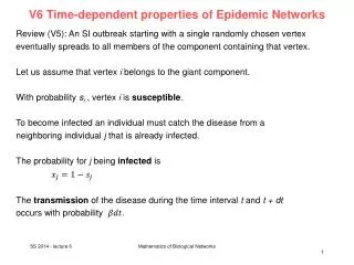
V6 Time- dependent properties of Epidemic Networks. Review (V5): An SI outbreak starting with a single randomly chosen vertex eventually spreads to all members of the component containing that vertex . Let us assume that vertex i belongs to the giant component .

E N D
V6 Time-dependentpropertiesofEpidemic Networks Review (V5): An SI outbreakstartingwith a singlerandomlychosenvertexeventuallyspreadsto all membersofthecomponentcontainingthatvertex. Letusassumethatvertexibelongstothegiantcomponent. Withprobabilitysi , vertexiissusceptible. Tobecomeinfected an individual must catch thediseasefrom a neighboring individual jthatisalreadyinfected. The probabilityforjbeinginfectedis The transmissionofthediseaseduringthe time intervaltandt + dt occurswithprobability. Mathematics of Biological Networks
Review: Time-dependentpropertiesofEpidemic Networks Multiplying theseprobabilitiesandthensummingover all neighborsofi , yieldsthe total probabilityofibecominginfected: whereAijis an elementoftheadjacencymatrix. Thus, thesiobey a setofn non-linear differential equations =- Fromwegetthecomplementaryequationforxi. = We will assumeagainthatthediseasestartseitherwith a singlevertex or a smallrandomlyselectednumbercofvertices. Thus xi = c/n→ 0, si = 1 - c/n→ 1 in thelimitfor large n. Mathematics of Biological Networks
Review: Time-dependentpropertiesofEpidemic Networks The equation=- is not solvable in closed form forgeneralAij. Byconsideringsuitablelimits, wecancalculatesomefeaturesofitsbehavior. Letus e.g. considerthebehaviorofthesystem at earlytimes. For large nandthegiven initial conditions, xi will besmall in thisregime. Byignoringtermsofquadraticorder, wecanapproximate or in matrix form wherexisthevectorwithelementsxi . Mathematics of Biological Networks
Review: Time-dependentpropertiesofEpidemic Networks Write xas a linear combinationoftheeigenvectorsoftheadjacencymatrix wherevristheeigenvectorwitheigenvaluer . Then Bycomparingterms in vrweget This hasthesolution Substitutingthisexpression back gives The fastest growingterm in thisexpressionisthetermcorresponding tothelargesteigenvalue1. Mathematics of Biological Networks
Review: Time-dependentpropertiesofEpidemic Networks Assuming thistermdominatesovertheotherswe will get So weexpectthenumberofinfectedindividualstogrowexponentially, just as in thefullymixedversionofthe SI model, but nowwith an exponentialconstantthatdepends not only on but also on theleadingeigenvalueoftheadjacencymatrix. The probabilityofinfection in thisearlyperiodvariesfromvertextovertex roughlyasthecorrespondingelementoftheleadingeigenvectorv1 . Mathematics of Biological Networks
Propagation of SI model on network Forlongtimes, thenetworkversionofthe SI modelpredictsthattheprobability ofinfectionofa vertex in thegiantcomponenttendsto 1. This isqualitativelysimilartothefullymixedversionofthe SI model. Whathappensifweintegratenumerically? The curve „first-order“ showstheresults of a numericalintegration. The pointslabelled„simulation“ areaverage valuesfrommanysimulationsofsimulated epidemicswiththe same spreading. → theagreementis ok but not perfect. Mathematics of Biological Networks
Propagation of SI model on network The reasonforthisdiscrepancyisthattheprobabilitiesofthetwonodesiandj in are not independent. In general, thequantitiessiandxjbetweenneighboringverticesarecorrelated. Wecanincorporatethisintoourcalculations, at least approximately, byusing a so-calledpair approximation. Mathematics of Biological Networks
Pair approximations Let usdenotebytheaverageprobabilitythatvertexiissusceptible. Similarly, is the averageprobabilitythatiisinfectedand is theaverageprobabilitythatiissusceptible AND jisinfected at the same time. This yieldsnow a trulyexactversionofourpreviouseq. (1) The previouslyusedequation is an approximationtothistrueequationwhereweassumedthat The troublewiththeneweq. isthatwecannotsolveitdirectlybecause itcontainstheunkownquantity. Mathematics of Biological Networks
Pair approximations -> weneed an expression for . Toreachthestatewhereiissusceptibleandjisinfected, j must havebeeninfectedbyanotherneighboringvertexk. The probabilityfor such a previousconfigurationwhereiandj aresusceptible andk isinfectedis. Whenstartingwiththisconfiguration, j will becomeinfected via kwith rate . Summingover all neighborskexceptfori, the total rate at whichj becomesinfectedis Mathematics of Biological Networks
Pair approximations However, can also decreasewhenibecomesinfected. This can happen in 2 ways. • Eithericanbeinfectedbyitsinfectedneighborjwhathappenswih rate or • icanbeinfectedbyanotherneighborl jso thatiisinfectedwith rate Summingthelatterexpressionover all neighborslotherthanjgives a total rate of Mathematics of Biological Networks
Pair approximations Putting all thesetermstogether, weget - In theorythisequationnowallowsustocalculate. In practice, itinvolvesyetmoretermsthatwedon‘tknow on theright-hand side, thethree-variable averages and . Such asuccessionofequations will never end – in thejargonofmathematics, itdoesn‘tclose. Mathematics of Biological Networks
Moment closure However, wecanmakeprogressbyapproximatingthe 3-variable averagesbyappropriatecombinationsof 1-variable and 2-variable averages. This will allowustoclosetheequationsandget a setthatwecansolve. This processiscalledmomentclosure. The momentclosuremethod at thelevelof 2-variable averagesthatwediscusshereis also calledpair approximationmethod. Startingwith- ourgoalistoapproximatethe 3-variable averageswithlower-order ones. Mathematics of Biological Networks
Moment closure We will makeuseofBayestheoremforprobabilities: wheremeanstheprobabilitythatvertexiis in thesetSofsusceptiblevertices. Weknowthatiandjareneighbors in thenetworkandthatjandkareneighbors. We will assumethatthediseasestateofkdoes not depend on thediseasestateofi. Iftheonlypath in thenetworkfromitokisthroughj,thisis a goodapproximation. Ifthereisanotherpath, thisremains an approximation. Mathematics of Biological Networks
Moment closure Assuming thestateofktobeindepdendentofthestateofi, wehave After puttingthisintoourpreviousequationweget In a similarway, wecanderive an expressionfortheother 3-variable average Mathematics of Biological Networks
Moment closure We cannowsubstitutebothexpressionsintoourpreviousequationandgetthe pair approximationequation This equationnowcontainsonlyaveragesover 2 variables at a time. Itcontains also a newaveragethatwehave not encounteredbefore. This canberewrittenas. Withthis, oureq. becomes (2) We will simplifythiseq. further. Mathematics of Biological Networks
Moment closure Let usdefinepijtobetheconditionalprobabilitythatjisinfectedgiventhati is not: Thenthe time evolutionofpijisgivenby The terms in the 2 sums overlnowcancel out exceptforl = j, leaving wherehave also usedAij = 1 Use (1) and (2) Mathematics of Biological Networks
Moment closure Rewriting in termsofpijgives whichhasthesolution Numericalintegrationofthese 2 equationsfor and givesthe „secondorder“ curve, whichagreesverynicelywith thesimulatedepidemics. Mathematics of Biological Networks 17
Recentextensions in modellingdiseasespreading Itisestimatedthatby 2030 morethan 60% oftheworld‘spopulation live in cities. Urban areas form a perfectfabricfor fast, uncontrolleddiseasepropagation. -> Need tomodel inter-person contacts in moredetailthanby differential equations. Nature 429, 180 (2004) Authorsusedthe Transportation Analysis and Simulation System (TRANSIMS) developed at Los AlamosNatl. Laboratories. Mathematics of Biological Networks 18
TRANSIMS TRANSIMS creates a syntheticpopulationwith a demographicdistribution (age, income) consistentwithjointdistributions in censusdata. The programuses an agent-basedparadigmtosimulatethemovementof all individualsduring e.g. oneday. Bythisitestimatespositionsandactivitiesof all travelersusing a transportationinfrastructure on a second-by-secondbasis. Nature 429, 180 (2004) Mathematics of Biological Networks 19
Model socialcontactnetworkasbipartitegraph a, A bipartite graph GPL with two types of vertices representing four people (P) and four locations (L). If person p visited location l, there is an edge in this graph between p and l. Vertices are labelled with appropriate demographic or geographic information, edges with arrival and departure times. For the city Portland / US, GPL has about 1.6 million vertices with a giant component of 1.5 million people and 180.000 locations. Nature 429, 180 (2004) Mathematics of Biological Networks 20
Degree distributions for estimated Portland social network. a, The number of people QPLj who visited j different locations in the bipartite people–locations graph GPL. On average people visited 4 locations / day. This distribution decays exponentially (nobody visited more than 15 locations in 1 day). b, The number of locations MPLi in GPL that are visited by exactly i different people. This plot follows a power-law tail. The slope of the straight-line graph is -2.8. Nature 429, 180 (2004) Mathematics of Biological Networks 21
Diseasetransmission Manyinfectiousdiseasesgettransmittedbetweenpeople in the same location. Diseasesspreadmainly due topeople‘smovement. -> investigatetwoprojectionsofGPLobtained by drawing an edge between all pairs of vertices that have a distance of 2 from each other on the bipartite graph. This yields two disconnected graphs GP and GL. Nature 429, 180 (2004) Mathematics of Biological Networks 22
Staticprojectionsofgraph GPL In GPthe edges are labelled with the sets of time intervals during which the people were co-located. For simplicity, we will discard these time labels and look at the static projections shown below d, People (such as 24-year-old male) are represented by filled circles, and locations (such as 34 Elm Street) by open squares. This projection yields a worst-case scenario for the spreading of a disease because the static graph is much more connected than GP. Consider also the idea of an “effective contact” by removing all edges for which the duration of contact was shorter than 1 hour. Nature 429, 180 (2004) Mathematics of Biological Networks 23
Degreedistributionsofstaticgraph d, The in and out degree distributions of the locations network GL. This network resembles a scale-free network with a power-law distribution. The slope of the straight-line graph is -2.8. c, The number of people who have kneighbors in the static people–contact graph P on log–log scale. This network resembles a small-world network. The scale-freenatureofthelocalizationnetworkreflectsthecapacitydistributionoflocations. Shopping mallstakeup large numbersofpeoplewhonormally live in smallhomes. Nature 429, 180 (2004) Mathematics of Biological Networks 24
Effectsofremoving high-degreevertices Can onee.g. preventdiseasepropagation in thissocialnetworkbyvaccinating (orputtingintoquarantine) a smallnumberof high-degreevertices? -> investigatethesizeofthegiantcomponent after removingfrom the bipartite graph GPLall verticeswithdegreehigherthank. -> evenwhen all verticesofdegree 11 andhigherareremoved, a uniquegiantcomponentpersists. Thus, anyeffectivevaccinationstrategy must bemassvaccination. Nature 429, 180 (2004) Mathematics of Biological Networks 25
Effectofremovingmostvisitedlocations In bwe remove all locations with degree k or higher from GPL and monitor the size of the largest connected component in the static people–contact graph induced by the remaining bipartite graph -> Even closingthe most-visitedlocations – orvaccinatingeveryonewhovisitsthem – does not shattertheinduced people-contactgraphuntil large fractionsofthepopulationhavebeeneffected. Q: Can epidemicsbestopped at all withoutresortingtomassvaccination? Nature 429, 180 (2004) Mathematics of Biological Networks 26
Early detection An alternative strategycouldinvolveearlydetectionofinfectedindividualsandefficienttargeting. Consideran idealizedsituation in whichsensors at a locationcandetectwhetheranypersonisinfected. The feasibilityofearlydetectiondepends on thenumberofsensorsrequired. This problemisequivalenttofindingtheminimumdominatingset. Nature 429, 180 (2004) Mathematics of Biological Networks 27
Overlapratio We wishto find a subset L‘ oflocations so that all (ormost) peoplevisitsomelocation in L‘. The overlapratio (J) of a setoflocations J L is wheren(J)isthe total numberofpeoplevisitinganylocation in J anddeg(l) isthenumberof different peoplevisitinglocationl J. The smallertheoverlapration, the larger isthenumberof different locations in J visitedby a singleperson. d. Overlapratiobydegree. The lowercurveshowsthe cumulativeoverlapratiobydegree, whichistheoverlapratio forlocationshavingdegree k orless. The uppercurveshows theoverlapratioforlocationshavingdegree = k. -> Not manypeoplevisitmorethanonehigh- degreelocationper day. Early detectioncould beaccomplishedbyplacingsensorsthere. Nature 429, 180 (2004) Mathematics of Biological Networks 28
Recentextensions in modellingdiseasespreading Use IATA database : 3880 airports , 18.810 weighted edges, where weight wjldenotes passenger flow between airports j and l. Consider also populations Nj of the metropolitan areas served by each airport. Focus on 3100 largest airports and 17182 edges accounting for 99% of the world-wide air traffic. PNAS 103, 2015 (2006) Mathematics of Biological Networks 29
Properties oftheworld-wideairportnetwork (B) The distribution of the weights (fluxes) is skewed and heavy-tailed. (A) The degree distribution P(k) that an airport j has kj connections to other airports follows a power-law behavior on almost two decades with exponent 1.8 ± 0.2. PNAS 103, 2015 (2006) Mathematics of Biological Networks 30
Properties oftheworld-wideairportnetwork (C) The distribution of populationsNjis heavy-tailed distributed. (D) The city population varies with the traffic of the corresponding airport as N ≈ Tα with α ≅ 0.5. PNAS 103, 2015 (2006) Mathematics of Biological Networks 31
Model diseasepropagrationby SIR modelforeachairport Use compartment model with 3100 compartments. In each city (airport), individuals can exist in one of 3 discrete states: susceptible (S), infected (I), permanently recovered (R) Model dynamics by numerical integration of a set of 3 3100 stochastic differential equations. PNAS 103, 2015 (2006) Mathematics of Biological Networks 32
Recentextensions in modellingdiseasespreading Geographical representation of the disease evolution in the United States for an epidemics starting in Hong Kong based on a SIR dynamics within each city. The color code corresponds to the prevalence in each region, from 0 to the maximum value reached (ρmax). Top row: the original United States maps, Bottom row: obtained by rescaling each region according to its population. Shown below are 3 representations of the airport network restricted to the 100 airports in the United States with highest traffic; the color is assigned in accordance to the color code adopted for the maps. PNAS 103, 2015 (2006) Mathematics of Biological Networks 33
Heterogeneityofepidemicpattern heterogeneity of epidemic pattern in actual network (WAN) is compared with 2network models (HOMN and HETN). HOMN: homogenous Erdos-Renyi random graph HETN: topology of real network For HOMN and HETN, all fluxes and populations are set to average value. Shown is entropy . H(t) = 1 means that epidemics is homogenously distributed over all nodes. H(t) = 0 means that only 1 city is affected Each profile is split into 3different phases. The central phase corresponds to H> 0.9; i.e., to a homogeneous geographical spread of the disease. This phase is much longer for the HOMN than for the real airport network WAN. The behavior observed in HETN is close to the real case meaning that the connectivity pattern plays a leading role in the epidemic behavior. PNAS 103, 2015 (2006) Mathematics of Biological Networks 34
Whatcitiesareaffected? Percentage of infected cities as a function of time for an epidemics starting in Hong Kong based on a SIR dynamics within each city. The HOMN case displays a large interval in which all cities are infected. The HETN and the real case show a smoother profile with long tails, signature of a long lasting geographical heterogeneity of the epidemic diffusion. PNAS 103, 2015 (2006) Mathematics of Biological Networks 35
Quality ofdiseaseforecasts? Measure similarity of 2 outbreak scenarios. Overlap = 1 means that the very same cities have the very same number of infectious individuals in both realizations. Overlap = 0 means that the two realizations do not have any common infected cities at time t. PNAS 103, 2015 (2006) Mathematics of Biological Networks 36
Overlapas a functionof time (Right): Outbreaks from poorly connected cities lead in all models to well reproducable behavior because only few connections are available. (Left): Outbreaks from hubs lead to well reproducable behavior in the HOMN model. The HETN and WAN models lead to considerable variation of the results here because the epidemics can take one of several possible channels. (Left): initially infected city is an airport hub (Right): initially infected city is a poorly connected city. PNAS 103, 2015 (2006) Mathematics of Biological Networks 37
Conclusions • air-transportation-network properties seems responsible for the global pattern of emerging diseases. • Large-scale mathematical models that take fully into account the complexity of the transportation matrix can be used to obtain detailed forecast of emergent disease outbreaks. • To make the forecast more realistic, it is necessary to introduce more details in the disease dynamics. In particular, seasonal effects and geographical heterogeneity in the basic transmission rate (due to different hygienic conditions and health care systems in different countries) should be addressed. • Also need to connect air transportation network with other transportation systems such as railways and highways for forecasting on longer time scales. PNAS 103, 2015 (2006) Mathematics of Biological Networks 38