Download
1 / 41
450 likes | 936 Vues
Iterative Improvement of a Solution to Linear Equations. When solving large sets of linear equations: Not easy to obtain precision greater than computer’s limit. Roundoff errors accumulation. There is a technique to recover the lost precision. Iterative Improvement.

E N D
Iterative Improvement of a Solution toLinear Equations • When solving large sets of linear equations: • Not easy to obtain precision greater than computer’s limit. • Roundoff errors accumulation. • There is a technique to recover the lost precision.
Iterative Improvement • Suppose that a vector Xis the exact solution of the linear set: …….(1) • Suppose after solving the linear set we get x with some errors (due to round offs) that is: • Multiplying this solution by A will give us b with some errors: ……(2)
Iterative Improvement • Subtracting (1) from (2) gives: ……(3) • Substituting (2) into (3) gives • All right-hand side is known and we to solve for δx.
Iterative Improvement • LU decomposition is calculated already, so we can use it. • After solving , we subtract δx from initial solution. • these steps can be applied iteratively until the convergence accrued.
Example results x[0]= -0.36946858035662183405989367201982531696557998657227 x[1]= 2.14706111638707763944466933025978505611419677734375 x[2]= 0.24684415554730337882816115779860410839319229125977 x[3]= -0.10502171013263031373874412111035780981183052062988 ------------------------------ r[0]= 0.00000000000000034727755418821271741155275430324117 r[1]= -0.00000000000000060001788899622500577609971306220602 r[2]= 0.00000000000000004224533421990125435980840581711310 r[3]= -0.00000000000000006332466855427798533040573922362522 ------------------------------ x[0]= -0.36946858035662216712680105956678744405508041381836 x[1]= 2.14706111638707808353387918032240122556686401367188 x[2]= 0.24684415554730332331700992654077708721160888671875 x[3]= -0.10502171013263024434980508203807403333485126495361 Initial solution Restored precisions Improved solution
SVD - Overview A technique for handling matrices (sets of equations) that do not have an inverse. This includes square matrices whose determinant is zero and all rectangular matrices. Common usages include computing the least-squares solutions, rank, range (column space), null space and pseudoinverse of a matrix.
SVD - Basics The SVD of a m-by-nmatrix A is given by the formula : Where : Uis a m-by-n matrix of the orthonormal eigenvectors of AAT VT is the transpose of a n-by-n matrix containing the orthonormal eigenvectors of ATA W is a n-by-n Diagonal matrix of the singular values which are the square roots of the eigenvalues of ATA
The Algorithm Derivation of the SVD can be broken down into two major steps [2] : • Reduce the initial matrix to bidiagonal form using Householder transformations • Diagonalize the resulting matrix using QR transformations Initial Matrix Bidiagonal Form Diagonal Form
Householder Transformations A Householder matrix is a defined as : H = I – 2wwT Where w is a unit vector with |w|2 = 1. It ends up with the following properties : H = HT H-1 = HT H2 = I (Identity Matrix) If multiplied by another matrix, it results in a new matrix with zero’ed elements in a selected row / column based on the values chosen for w.
Applying Householder To derive the bidiagonal matrix, we apply successive Householder matrices :
Application con’t From here we see : P1M = M1 M1S1 = M2 P2M2 = M3 …. MNSN = B [If M > N, then PMMM = B] This can be re-written in terms of M : M = P1TM1 = P1TM2S1T = P1TP2TM3S1T = … = P1T…PMTBSNT…S1T = P1…PMBSN…S1 (Because HT = H)
Householder Derivation Now that we’ve seen how Householder matrices are used, how do we get one? Going back to its definition : H = I – 2wwT Which is defined in terms of w - which is defined as To make the Householder matrix useful, w must be derived from the column (or row) we want to transform. This is accomplished by setting xto row / column to transform and y to desired pattern. and and (Length operator)
Householder Example To derive P1 for the given matrix M : We would have : With : • This leads to : • Simplifying : • Then :
Example con’t • Finally : • With that : • Which we can see zero’ed the first column. • P1 can be verified by performing the reverse operation :
Example con’t Likewise the calculation of S1 for : Would have : With : • This leads to : • Then :
Example con’t • Finally : • With that : • Which we can see zero’ed the first row.
The QR Algorithm As seen, the initial matrix is placed into bidiagonal form which results in the following decomposition : M = PBS with P = P1...PNand S = SN…S1 The next step takes B and converts it to the final diagonal form using successive QRtransformations.
QR Decompositions The QR decomposition is defined as : M = QR Where Q is an orthogonal matrix (such that QT = Q-1, QTQ = QQT = I) And R is an upper triangular matrix : It has the property such that RQ = M1to which another decomposition can be performed. Hence M1 = Q1R1,R1Q1= M2 and so on.In practice, after enough decompositions, Mxwill converge to the desired SVD diagonal matrix – W.
QR Decomposition con’t Because Q is orthogonal (meaning QQT = QTQ = 1), we can redefine Mx in terms of Qx-1 and Mx-1only : Which can be written as : Starting with M0= M, we can describe the entire decomposition of W as : One question remains – How do we derive Q? Multiple methods exist for QR decompositions – including Householder Transformations, Hessenberg Transformations, Given’s Rotations, Jacobi Transformations, etc. Unfortunately the algorithm from book is not explicit on its chosen methodology – possibly Givens as it is used by reference material.
QR Decomposition using Givens rotations A Givens rotation is used to rotate a plane about two coordinates axes and can be used to zero elements similar to the householder reflection. It is represented by a matrix of the form : The multiplication GTA* effects only the rows i and j in A. Likewise the multiplication AG only effects the columns i and j. [1] Shows transpose on pre-multiply – but examples do not appear to be transposed (i.e. –s is still located i,j).
Givens rotation The zeroing of an element is performed by computing the c and s in the following system. Where b is the element being zeroed and a is next to b in the preceding column / row. This is results in :
Givens rotation and the Bidiagonal matrix The application of Givens rotations on a bidiagonal matrix looks like the following and results in its implicit QR decomposition.
Givens and Bidiagonal With the exception of J1, Jx is the Givens matrix computed from the element being zeroed. J1 is computed from the following : Which is derived from B and the smallest eigenvalue (λ) of T
Bidiagonal and QR This computation of J1 causes the implicit formation of BTB which causes :
QR Decomposition Given's rotationexample Ref: An example of QR Decomposition, Che-Rung Lee, November 19, 2008
QR Decomposition Given's rotationexample Ref: An example of QR Decomposition, Che-Rung Lee, November 19, 2008
QR Decomposition Given's rotationexample Ref: An example of QR Decomposition, Che-Rung Lee, November 19, 2008
QR Decomposition Given's rotationexample Ref: An example of QR Decomposition, Che-Rung Lee, November 19, 2008
QR Decomposition Given's rotationexample Ref: An example of QR Decomposition, Che-Rung Lee, November 19, 2008
QR Decomposition Given's rotationexample Ref: An example of QR Decomposition, Che-Rung Lee, November 19, 2008
QR Decomposition Given's rotationexample Ref: An example of QR Decomposition, Che-Rung Lee, November 19, 2008
Putting it together - SVD Starting from the beginning with a matrix M, we want to derive - UWVT Using Householder transformations : [Step 1] Using QR Decompositions : [Step 2] Substituting step 2 into 1 : With U being derived from : And VT being derived from : Which results in the final SVD :
SVD Applications Calculation of the (pseudo) inverse : [1] : Given [2] : Multiply by M-1 [3] : Multiply by V [4]* : Multiply by W-1 [5] : Multiply by UT [6] : Rearranging *Note – Inverse of a diagonal matrix is diag(a1,…,an)-1 = diag(1/a1,…,1/an)
SVD Applications con’t Solving a set of homogenous linear equations i.e. Mx = b Case 1 : b = 0 x is known as the nullspace of M which is defined as the set of all vectors that satisfy the equation Mx = 0. This is any column in VT associated with a singular value (in W) equal to 0. Case 2 : b != 0 Then we have : Which can be re-written as : From the previous slide we know : Hence : which is easily solvable
SVD Applications con’t Rank, Range, and Null space • The rank of matrix A can be calculated from SVD by the number of nonzero singular values. • The range of matrix A is The left singular vectors of U corresponding to the non-zero singular values. • The null space of matrix A is The right singular vectors of V corresponding to the zeroed singular values.
SVD Applications con’t Condition number • SVD can tell How close a square matrix A is to be singular. • The ratio of the largest singular value to the smallest singular value can tell us how close a matrix is to be singular: • A is singular if c is infinite. • A is ill-conditioned if c is too large (machine dependent).
SVD Applications con’t Data Fitting Problem
SVD Applications con’t Image processing [U,W,V]=svd(A) NewImg=U(:,1)*W(1,1)*V(:,1)’
SVD Applications con’t Digital Signal Processing (DSP) • SVD is used as a method for noise reduction. • Let a matrix A represent the noisy signal: • compute the SVD, • and then discard small singular values of A. • It can be shown that the small singular values mainly represent the noise, and thus the rank-k matrix Akrepresents a filtered signal with less noise.
Additional References • Golub & Van Loan – Matrix Computations; 3rd Edition, 1996 • Golub & Kahan – Calculating the Singular Values and Pseudo-Inverse of a Matrix; SIAM Journal for Numerical Analysis; Vol. 2, #2; 1965 • An Example of QR Decomposition, Che-Rung Lee, November 19, 2008