Iterative Solution Methods
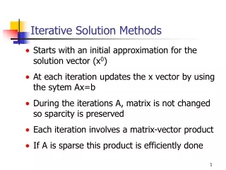
Iterative Solution Methods. Starts with an initial approximation for the solution vector (x 0 ) At each iteration updates the x vector by using the sytem Ax=b During the iterations A, matrix is not changed so sparcity is preserved Each iteration involves a matrix-vector product

Iterative Solution Methods
E N D
Presentation Transcript
Iterative Solution Methods • Starts with an initial approximation for the solution vector (x0) • At each iteration updates the x vector by using the sytem Ax=b • During the iterations A, matrix is not changed so sparcity is preserved • Each iteration involves a matrix-vector product • If A is sparse this product is efficiently done
Iterative solution procedure • Write the system Ax=b in an equivalent form x=Ex+f (like x=g(x) for fixed-point iteration) • Starting with x0, generate a sequence of approximations {xk} iteratively by xk+1=Exk+f • Representation of E and f depends on the type of the method used • But for every method E and f are obtained from A and b, but in a different way
Convergence • As k, the sequence {xk} converges to the solution vector under some conditions on E matrix • This imposes different conditions on A matrix for different methods • For the same A matrix, one method may converge while the other may diverge • Therefore for each method the relation between A and E should be found to decide on the convergence
Different Iterative methods • Jacobi Iteration • Gauss-Seidel Iteration • Successive Over Relaxation (S.O.R) • SOR is a method used to accelerate the convergence • Gauss-Seidel Iteration is a special case of SOR method
Dxk+1 xk+1=Exk+f iteration for Jacobi method A can be written as A=L+D+U (not decomposition) Ax=b (L+D+U)x=b Dxk+1 =-(L+U)xk+b xk+1=-D-1(L+U)xk+D-1b E=-D-1(L+U) f=D-1b
Use the latest update Gauss-Seidel (GS) iteration
Dxk+1 x(k+1)=Ex(k)+f iteration for Gauss-Seidel Ax=b (L+D+U)x=b (D+L)xk+1 =-Uxk+b xk+1=-(D+L)-1Uxk+(D+L)-1b E=-(D+L)-1U f=-(D+L)-1b
Comparison • Gauss-Seidel iteration converges more rapidly than the Jacobi iteration since it uses the latest updates • But there are some cases that Jacobi iteration does converge but Gauss-Seidel does not • To accelerate the Gauss-Seidel method even further, successive over relaxation method can be used
Correction term Multiply with Successive Over Relaxation Method • GS iteration can be also written as follows Faster convergence
SOR 1<<2 over relaxation (faster convergence) 0<<1 under relaxation (slower convergence) There is an optimum value for Find it by trial and error (usually around 1.6)
x(k+1)=Ex(k)+f iteration for SOR Dxk+1=(1-)Dxk+b-Lxk+1-Uxk (D+ L)xk+1=[(1-)D-U]xk+b E=(D+ L)-1[(1-)D-U] f= (D+ L)-1b
The Conjugate Gradient Method • Converges if A is a symmetric positive definite matrix • Convergence is faster
Substitute this into Convergence of Iterative Methods Define the solution vector as Define an error vector as
Convergence of Iterative Methods power iteration The iterative method will converge for any initial iteration vector if the following condition is satisfied Convergence condition
Norm of a vector A vector norm should satisfy these conditions Vector norms can be defined in different forms as long as the norm definition satisfies these conditions
Commonly used vector norms Sum norm or ℓ1 norm Euclidean norm or ℓ2 norm Maximum norm or ℓ norm
Norm of a matrix A matrix norm should satisfy these conditions Important identitiy
Commonly used matrix norms Maximum column-sum norm or ℓ1 norm Spectral norm or ℓ2 norm Maximum row-sum norm or ℓ norm
17 13 15 16 19 10 Example • Compute the ℓ1 and ℓ norms of the matrix
Convergence condition Express E in terms of modal matrix P and :Diagonal matrix with eigenvalues of E on the diagonal
is a sufficient condition for convergence Sufficient condition for convergence If the magnitude of all eigenvalues of iteration matrix E is less than 1 than the iteration is convergent It is easier to compute the norm of a matrix than to compute its eigenvalues
Convergence of Jacobi iteration E=-D-1(L+U)
Convergence of Jacobi iteration Evaluate the infinity(maximum row sum) norm of E Diagonally dominant matrix If A is a diagonally dominant matrix, then Jacobi iteration converges for any initial vector
Stopping Criteria • Ax=b • At any iteration k, the residual term is rk=b-Axk • Check the norm of the residual term ||b-Axk|| • If it is less than a threshold value stop
Example 1 (Jacobi Iteration) Diagonally dominant matrix
Example 1 continued... Matrix is diagonally dominant, Jacobi iterations are converging
Example 2 The matrix is not diagonally dominant
Example 2 continued... The residual term is increasing at each iteration, so the iterations are diverging. Note that the matrix is not diagonally dominant
Convergence of Gauss-Seidel iteration • GS iteration converges for any initial vector if A is a diagonally dominant matrix • GS iteration converges for any initial vector if A is a symmetric and positive definite matrix • Matrix A is positive definite if xTAx>0 for every nonzero x vector
Positive Definite Matrices • A matrix is positive definite if all its eigenvalues are positive • A symmetric diagonally dominant matrix with positive diagonal entries is positive definite • If a matrix is positive definite • All the diagonal entries are positive • The largest (in magnitude) element of the whole matrix must lie on the diagonal
Not positive definite Largest element is not on the diagonal Not positive definite All diagonal entries are not positive Positive Definitiness Check Positive definite Symmetric, diagonally dominant, all diagonal entries are positive
Positive Definitiness Check A decision can not be made just by investigating the matrix. The matrix is diagonally dominant and all diagonal entries are positive but it is not symmetric. To decide, check if all the eigenvalues are positive
Jacobi iteration Example (Gauss-Seidel Iteration) Diagonally dominant matrix
Jacobi iteration Example 1 continued... When both Jacobi and Gauss-Seidel iterations converge, Gauss-Seidel converges faster
Convergence of SOR method • If 0<<2, SOR method converges for any initial vector if A matrix is symmetric and positive definite • If >2, SOR method diverges • If 0<<1, SOR method converges but the convergence rate is slower (deceleration) than the Gauss-Seidel method.
Operation count • The operation count for Gaussian Elimination or LU Decomposition was 0 (n3), order of n3. • For iterative methods, the number of scalar multiplications is 0 (n2) at each iteration. • If the total number of iterations required for convergence is much less than n, then iterative methods are more efficient than direct methods. • Also iterative methods are well suited for sparse matrices