Basic Iterative Methods and Multigrid Ideas
Basic Iterative Methods and Multigrid Ideas. Hector D. Ceniceros Department of Mathematics UCSB Math 104 B. Material Based on “A Multigrid Tutorial” by W. L. Briggs and the “Multigrid Tutorial” by Livne. The problem: Solve the large linear system.

Basic Iterative Methods and Multigrid Ideas
E N D
Presentation Transcript
Basic Iterative Methods and Multigrid Ideas Hector D. Ceniceros Department of Mathematics UCSB Math 104 B Material Based on “A Multigrid Tutorial” by W. L. Briggs and the “Multigrid Tutorial” by Livne.
The problem: Solve the large linear system Iterative methods take the general matrix form: Convergence iff Iterative Methods Matrix form is good for analysis:
Examples of Iterative Methods In actual application of these methods we don’t use these matrices Instead we use equivalent forms for the iterations.
From Jacobi to GS Gauss-Seidel: Use the approximations as they are available:
SOR We can write SOR in the equivalent form Updated residual
Example 2: A BVP Introduce a grid and use finite differences
2 æ ö + c - 2 h 1 f æ ö v 1 ç ÷ æ ö 1 ç ÷ ç ÷ 2 ç ÷ - + c - f 1 2 h 1 v ç ÷ 2 2 ç ÷ ç ÷ ç ÷ ç ÷ v ç ÷ 2 1 f - + c - 1 2 h 1 3 3 ç ÷ ç ÷ ç ÷ 2 ç ÷ ç ÷ h ç ÷ v ç ÷ ç ÷ ç ÷ f - 2 N 2 - 2 - + c - N ç ÷ 1 2 h 1 ç ÷ ç ÷ v è ø - 1 N ç ÷ f è ø - 2 1 N - + c 1 2 h è ø A Tridiagonal System =
Basic Loop for Jacobi Jacobi. v0 stores the old (k) values. v stores the new (k+1) values j index is shifted by one. … while ( dif > TOL & iter <= MAX_ITER) for j=2:N v(j) =(v0(j-1) + v0(j+1) + f(j))/d; end iter=iter+1; dif=norm(v-v0,inf)/norm(v,inf); v0=v; end d=2+c*h^2
Basic Loop for GS … while ( dif > TOL & iter <= MAX_ITER) for j=2:N v(j) =(v(j-1) + v0(j+1) + f(j))/d; end iter=iter+1; dif=norm(v-v0,inf)/norm(v,inf); v0=v; end
Basic Loop for SOR …. while ( dif > TOL & iter <= MAX_ITER) for j=2:N v(j) =(1-w)*v0(j) + (w/d)*(f(j) + v(j-1) + v0(j+1)); end iter=iter+1; dif=norm(v-v0,inf)/norm(v,inf); v0=v; end
K=3 K=1 K=6 Performance of the Basic Iterative Methods We consider the BVP with f=0 and c=0. In this case the Exact solution of Ax=b is the x=0. We use Fourier modes as initial guesses
Error vs Iterations Jacobi Gauss-Seidel SOR Error decreases fast for large k but slowly for small k!
Error reduction stalls Jacobi: Initial guess: p p p j 6 j 3 2 j æ æ ö æ ö æ ö ö 1 = + + v s i n s i n s i n ç ç ÷ ç ÷ ç ÷ ÷ 0 3 N N N è è ø è ø è ø ø | | | | e ¥
p p p 2 j 1 6 j 3 2 j æ ö æ ö æ ö 1 1 = + + v s i n s i n s i n ç ÷ ç ÷ ç ÷ j N 2 N 2 N è ø è ø è ø Jacobi, GS Relaxation Smooth the Error • Initial error: • Error after 35 iteration sweeps: Many relaxation schemes have the smoothing property: oscillatory modes of the error are eliminated effectively, but smooth modes are damped very slowly.
Observation Toward Multigrid • Many relaxation schemes have the smoothing property, where oscillatory modes of the error are eliminated effectively, but smooth modes are damped very slowly. • This might seem like a limitation, but by using coarse grids we can use the smoothing property to good advantage. What is smooth on fine grid looks rougher on a coarser grid
Smooth Error is (relatively) more Oscillatory on Coarse Grid • A smooth function: • Can be represented by linear interpolation from a coarser grid:
Another Observation for Multigrid Let v be an approximation to the solution of Au=f, where the residual r=f-Av. The the error e=u-v satisfies Ae=r. Thus if we have an approximation to the error e we can “correct” the approximation v by v’ = v +e This is called error or residual (coarse-grid) correction
Relaxing Ae=r • After relaxing on Au=f on the fine grid, the error will be smooth. On the coarse grid, however, this error appears more oscillatory, and relaxation will be more effective. • Therefore we go to a coarse grid and relax on the residual equation Ae=r, with an initial guess of e=0.
Restrict Coarse-grid Correction Correct h h h Relax on = A u f h h h ¬ + u u e h h h h = - r f A u Compute Interpolate h 2 h h » e I e 2 h 2 h 2 h 2 h = A e r Solve
Multigrid • Coarse grid correction at multiple levels (nested iteration). • When multigrid converges (A positive definite, for example) is hard to beat. It yields the solution to Ax=b in O(N) operations, which is optimal.

