RT solution methods
RT solution methods. Review: What are we doing again?. Divide vertical, plane-parallel atmosphere up into approximately homogeneous sections. Calculate (composite) optical properties of each layer: τ , ϖ , PF( Θ ) at some wavelength λ . Monochhromatic !!

RT solution methods
E N D
Presentation Transcript
Review: What are we doing again? • Divide vertical, plane-parallel atmosphere up into approximately homogeneous sections. • Calculate (composite) optical properties of each layer: τ, ϖ, PF(Θ) at some wavelength λ. Monochhromatic!! • Goal: Calculate Total Intensities in any direction (θ,ϕ) at any τ(z). Typically τ=0, and τ=τ* (surface & TOA). • Sum over mu-weighted intensities to calculate (monochromatic) fluxesif desired. I+TOA(θ,ϕ) τ1, ϖ1, PF1(Θ) τ2, ϖ2, PF2(Θ) … … τn, ϖn, PFn(Θ)
Review: What are we doing again? I+TOA(θ,ϕ) • Divide vertical, plane-parallel atmosphere up into approximately homogeneous sections. • Calculate (composite) optical properties of each layer: τ, ϖ, PF(Θ) at some wavelength λ. Monochhromatic!! • Goal: Calculate Total Intensities in any direction (θ,ϕ) at any τ(z). Typically τ=0, and τ=τ* (surface & TOA). • Sum over mu-weighted intensities to calculate (monochromatic) fluxesif desired. τ1, ϖ1, PF1(Θ) τ2, ϖ2, PF2(Θ) … … τn, ϖn, PFn(Θ)
How do we do it? “Adding-Doubling” STEPS (for a given azimuthal moment m) • Use Doubling to calculate the properties R,T,s+,s- from the optical properties τ1, ϖ1, PF1(Θ) of each homogeneous layer. • Note: The source terms s+, s- can include both thermal and solar contributions. • Use Addingto calculate Rab, Rba, Tab, Tba, s+,s-of the full atmosphere. • Calculate the surface reflectance matrix Rg and source s+g (thermal+solar). • Combine the atmosphere & surface to calculate Im(μ) upwelling at TOA and downwelling at surface. • Calculate I in any direction upwelling@TOA, downwelling@surf:
So what did we calculate? • Monochromatic Intensity Iλat chosen observation angles (θ,ϕ) at surface (upwelling) or TOA (downwelling) • Easily extended to calculate at any level in atmosphere. • Can easily calculate fluxes from Im=0quantities. • Would need to repeat this for multiple wavelengths. • We assumed Plane-Parallel! • We only calculated Total Intensity I, not polarization!!
DISORT : 1988 • First really stable, easily available full scattering code (in Fortran 77) • Many codes are derivatives of this in one way or another since then. • And some people still use it!
Wiscombe RT contributions • DISORT - first publicly available N-stream multiple-scattering solar+thermal code. • Delta-Eddington for climate calculations • Fast, Stable Mie calculations, especially for large size parameter x (100-1000). • Delta-M phase function similarity transformation for large particle scattering (large forward scattering peak) • Adding-doubling and doubling initialization • Now he studies climate and exoplanets at NASA-Goddard.
Wiscombe RT contributions • DISORT - first publicly available N-stream multiple-scattering solar+thermal code. • Delta-Eddington for climate calculations • Fast, Stable Mie calculations, especially for large size parameter x (100-1000). • Delta-M phase function similarity transformation for large particle scattering (large forward scattering peak) • General doubling rules for variable temperature and solar sources. • Thin-layer initialization for doubling • Now he studies climate and exoplanets at NASA-Goddard.
Similarity Transformations: “Delta scaling” • For Highly forward-peaked phase functions (i.e., large size parameter x) “Truncation and renormalization” Water cloud phase function, 500 nm
Similarity Transformations: “Delta scaling” • Delta-M scaling introduced by Wiscombe much more robust. * Notes taken from K.F. Evans, http://nit.colorado.edu/atoc5560/
Similarity Transformations: “Delta scaling” *Note that these χl values are in the “Wiscombe” convention, where:
Similarity Transformations: “Delta scaling” • Can have nontrivial (few %) errors for solar radiances, but is very accurate for fluxes. • Still the errors are almost always much larger when you don’t use it! • An simple improvement introduced by Najakima & Tanaka (1988) reduces the intensity errors to ~0.1%.
The Eddington Approximation This is analytically solvable for I0 and I1. Solutions look like:
The Delta-Eddingtonapproximation is exactly this but using Delta-Scaling for f=g2.
“Successive Orders of Scattering” aka Neumann’s iterative solution
“Successive Orders of Scattering” • Keep track of # of times a stream is scattered. • Usually cut off after radiance at some location and angle has stopped changed. • For small amounts of scattering, will be small. • For large amounts of scattering, may have to keep track of 100s of scattering “orders” • IMPLEMENTATION • Divide layers into small enough layers so the source function of each layer does NOT require multiple scattering. • Use principle of interaction to propagate radiation. • Often is slow, especially for highly scattering atmospheres.
Rayleigh scattering • How many times is light scattered in a clear sky that reaches our eye?
Rayleigh scattering • How many times is light scattered in a clear sky that reaches our eye?
Cloud Scattering • Cloud with Optical Depth = 10, ϖ=1, g=0.85. • Downwelling Intensity (aziumthally-aveaged)
Microwave Rain Cases (Smith et al 2002, IEEE) Case 2: Low water, high ice ~ 0.3 mm/hr Case 1: Low water, low ice ~ 1 mm/hr Case 3: High water, low ice ~ 10 mm/hr Case 4: High water,High ice ~ 90 mm/hr * Note that surface reflection does NOT change the order of scattering in this case; only atmospheric scattering does.
Other Techniques:What can they do? • Some are 1D plane-parallel, quadrature-type methods simply to speed up the calculations: • “Eigenmatrix” Approach to find R, T of a homogeneous layer with larger optical depth (much faster than doubling) • Analytic solution available for 4-stream methods (Liou, 1980s) • Work here to speed up the eigenmatrix technique with “Pade Approximants” (McGarragh & Gabriel, 2010, 2013) • Delta-Eddington / Analytic 2-stream : very, very fast! • Some give you derivatives as well • “Tangent-Linear”: Change of the output with a given set of small input changes. • “Adjoint” : How much would each input need to change to yield a prescribed change in the output? • These are needed typically in many retrieval algorithms as well as data assimilation.
Other Techniques:What can they do? • Some provide additional insights: • Successive order of scattering provides how the radiance is distributed vs. scattering order. • Some codes give you radiances at intermediate levels- useful for varying aircraft observations. • Some codes are optimized for (spectral) fluxes rather than radiances. • 1D Monte-Carlo codes calculate the same quantities but are excellent as “truth” or a benchmark. Can make very pretty pictures of scattering as well!!
Monte-Carlo Techniques • Forward methods (generally solar only) launch photons from the sun and track them wherever they go. • If a photon makes it through a layer. If so, keep going. • If not, did it get absorbed or scattered? A new r. • r < ϖ : scattered. r > ϖ : absorbed. • If scattered, which direction did it go? Must know the Cumulative Probability of scattering less than a certain angle, based on the layer’s scattering phase function. • Can spin the emergent direction arbitrarily on (0,2π) about the incoming direction. So select a relative azimuth on (0,2π) • Repeat until photon absorbed, or makes it out. • If made it out, record direction • Number of photons per unit solid angle emerging in a given direction is proportional to intensity. • Can also be used for 3D calculations. • Output error is proportional to 1/sqrt(N), where N is the number of photons launched.
Reverse Monte-Carlo • Forward Monte-Carlo: most of the photons we launched are not interesting to us as they would not have made it to our detector. But if we care about the distribution of all photons – this is the way to go! • Reverse Monte-Carlo launches photons from the sensor rather than the sun, so needs far fewer photons to calculate the intensity in a given observation direction. • Works well in the thermal IR / microwave (azimuthal symmetry simplifies some of the calculations). • Can also be extended into the solar.
Reverse Monte-Carlo • Uses “time-reversal symmetry” of photons / RT equation: Photons travelling backwards in time act exactly the same as travelling forwards! • Launch photons from a sensor in the direction of observation. • Do everything pretty much the same, but this way only the photons you care about count. • For thermal: when it is absorbed at the atmosphere or surface, we know “where that photon came from” and assign it Bλ(T), for the temperature where it got absorbed. • Works well for 3D!
Monte-Carlo depictions of photons incident on an optical depth cloud layer
Other Techniques:What can they do? • Some solve much harder problems: • 3D methods – Can deal with horizontal inhomogeneity. • Independent Pixel Approximation • Slant Methods • Full 3D with horizontal photon transport. • Vector calculations: Include effects of polarization, calculate Stokes vectors. • Matrices generally becomes (4n, 4n) instead of (n,n) • Calculations become ~ 100x slower typically! • Curvature of Atmosphere • Important for very oblique or limb observations. (>80 deg) • “Pseudo-spherical” approximation is typical.
3D Effects in the Vis/NIR 06 UTC 09 UTC 12 UTC 15 UTC 18 UTC Courtesy P.M. Kostka