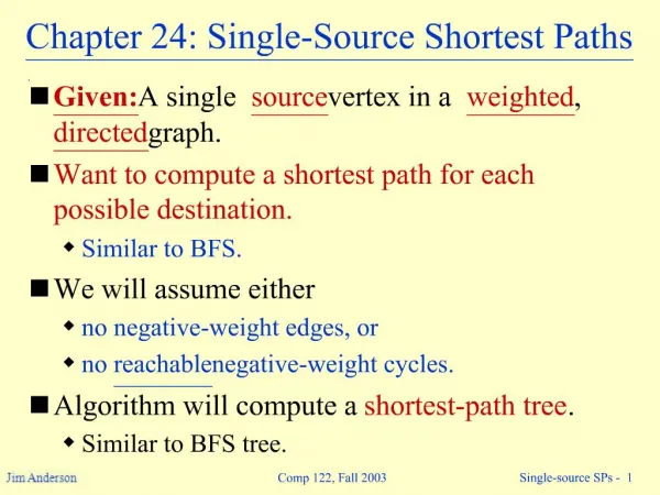
Single-Source Shortest Paths
Single-Source Shortest Paths. Contents. Definition Optimal substructure of a shortest path Negative-weight edges Cycles Predecessor subgraph Relaxation The Bellman-Ford algorithm Single-source shortest paths in directed acyclic graphs Dijkstra's algorithm. Definition. Definition

Single-Source Shortest Paths
E N D
Presentation Transcript
Contents • Definition • Optimal substructure of a shortest path • Negative-weight edges • Cycles • Predecessor subgraph • Relaxation • The Bellman-Ford algorithm • Single-source shortest paths in directed acyclic graphs • Dijkstra's algorithm
Definition • Definition • edge weight • path weight • shortest-path weight: δ(u,v) • shortest path
Definition • source, destination • single-source single-destination • single-source • single-destination • all pair
Optimal substructure of a shortest path • Optimal substructure of a shortest path • the shortest path consists of shortest subpath
Optimal substructure of a shortest path • Lemma 24.1 • Given a weighted, directed graph G = (V, E) with weight function w : E → R, let p = v1,v2,..., vk be a shortest path from vertex v1 to vkand, for any i and j such that 1 ≤ i ≤ j ≤k, let pij= vi, vi+1,..., vj be the subpath of p from vertex vito vj. Then, pijis a shortest path from vito vj.
Optimal substructure of a shortest path • Proof • If we decompose path p into , v1 vivj vk then we have that w(p) = w(p1i) + w(pij) +w(pjk). Now, assume that there is a path from vito vjwith weight w(p′ij)< w(pij). Then, v1 vivj vk is a path from v1 to vkwhose weight w(p1i)+w(p′ij)+w(pjk) is less than w(p), which contradicts the assumption that p is a shortest path from v1 to vk. p1i pij pjk p1i pij pjk
Negative-weight edges • Negative-weight edges • Negative-weight edges are permitted if negative-weight cycles are not reachable from s. b a -4 i h 3 -1 2 ∞ ∞ 4 3 g c s d 6 8 5 3 0 5 11 -∞ -8 -3 ∞ 2 f e 7 3 j -∞ -∞ -6 Figure 24.1
Cycles • Cycles • A shortest path does not include cycles. • A shortest path is of length at most |V|-1.
Predecessor subgraph • Predecessor subgraph • shortest-path tree • for example : shows a weighted , directed graph and two shortest-paths trees with the same root.
Predecessor subgraph t x 6 3 9 3 4 2 1 s 0 2 7 3 5 5 11 6 y z Figure 24.2 (a)
Predecessor subgraph t x 6 3 9 3 4 2 1 s 0 2 7 3 5 5 11 6 y z Figure 24.2 (b)
Predecessor subgraph t x 6 3 9 3 4 2 1 s 0 2 7 3 5 5 11 6 y z Figure 24.2 (c)
Relaxation • Relaxation • definition • path-relaxation property u v u v 2 2 9 6 5 5 Relax(u,v,w) Relax(u,v,w) u v u v 2 2 7 6 5 5
The Bellman-Ford algorithm • The Bellman-Ford algorithm • Running time : O(VE) • it solves the single source shortest-paths problem in the general case in which edge weights may be negative.
5 5 t t x x -2 -2 6 ¥ ¥ ¥ 6 6 -3 -3 8 8 s 0 s 0 7 7 -4 -4 2 2 7 7 7 ¥ ¥ ¥ 9 9 y z y z The Bellman-Ford algorithm • order • (t,x), (t,y), (t,z), (x,t), (y,x), (y,z), (z,x), (z,s), (s,t), (s,y)
5 5 t t x x -2 -2 6 4 2 4 6 6 -3 -3 8 8 s 0 s 0 7 7 -4 -4 2 2 7 7 7 2 7 2 9 9 y z y z The Bellman-Ford algorithm • order • (t,x), (t,y), (t,z), (x,t), (y,x), (y,z), (z,x), (z,s), (s,t), (s,y)
t x -2 2 4 6 -3 8 s 0 7 -4 2 7 7 -2 9 y z The Bellman-Ford algorithm • order • (t,x), (t,y), (t,z), (x,t), (y,x), (y,z), (z,x), (z,s), (s,t), (s,y) 5
Single-source shortest paths in directed acyclic graphs • Single-source shortest paths in directed acyclic graphs • Running time : O(V+E) time • starts by topologically sorting the dag to impose a linear ordering on the vertices. • just one pass over the vertices
Single-source shortest paths in directed acyclic graphs 6 1 y r s t x z 7 -1 5 2 -2 ∞ 0 ∞ ∞ ∞ ∞ 4 3 2 6 1 y s t x z r 7 -1 5 2 -2 ∞ 0 ∞ ∞ ∞ ∞ 4 3 2
Single-source shortest paths in directed acyclic graphs 6 1 y r s t x z 7 -1 5 2 -2 ∞ 0 2 6 ∞ ∞ 4 3 2 6 1 y s t x z r 7 -1 5 2 -2 ∞ 0 2 6 6 4 4 3 2
Single-source shortest paths in directed acyclic graphs 6 1 y r s t x z 7 -1 5 2 -2 ∞ 0 2 6 5 4 4 3 2 6 1 y s t x z r 7 -1 5 2 -2 ∞ 0 2 6 5 3 4 3 2
Single-source shortest paths in directed acyclic graphs 6 1 y r s t x z 7 -1 5 2 -2 ∞ 0 2 6 5 3 4 3 2
Dijkstra's algorithm • Dijkstra's algorithm • all edge weights are nonnegative. • the running time of Dijkstra's algorithm is lower than that of the Bellman-Ford algorithm. • Running time : • O (V^2) if we use array • O(VlgV + ElgV) if we use a heap • (VlgV + E) if we use a Fibonacci heap.
Dijkstra's algorithm DIJKSTRA(G, w, s) 1 INITIALIZE-SINGLE-SOURCE(G, s) 2 S ← Ø 3 Q ← V[G] 4 while Q ≠ Ø 5 do u ← EXTRACT-MIN(Q) 6 S ← S {u} 7 for each vertex v Adj[u] 8 do RELAX(u, v, w)
Dijkstra’s Algorithm t x 1 Q ∞ ∞ 10 9 2 3 4 6 s 0 5 7 ∞ ∞ 2 y z S
Dijkstra’s Algorithm t x 1 Q 10 ∞ 10 9 2 3 4 6 s 0 5 7 5 ∞ 2 y z {s} S
Dijkstra’s Algorithm t x 1 Q 10 ∞ 10 9 2 3 4 6 s 0 5 7 5 ∞ 2 y z {s, y} S
Dijkstra’s Algorithm t x 1 Q 8 14 10 9 2 3 4 6 s 0 5 7 5 7 2 y z {s, y} S
Dijkstra’s Algorithm t x 1 Q 8 13 10 9 2 3 4 6 s 0 5 7 5 7 2 y z {s, y, z, t} S
Dijkstra’s Algorithm t x 1 Q 8 9 10 9 2 3 4 6 s 0 5 7 5 7 2 y z {s, y, z, t} S
Dijkstra’s Algorithm t x 1 Q 8 9 10 9 2 3 4 6 s 0 5 7 5 7 2 y z {s, y, z, t, x} S