Shortest Paths in Weighted Directed Graphs
300 likes | 417 Vues
Learn about algorithms for finding the shortest path from a source vertex to all other vertices in a weighted directed graph. Explore various approaches, including Dijkstra's algorithm, Bellman-Ford algorithm, and solving the problem for unweighted graphs using Breadth-First Search (BFS).

Shortest Paths in Weighted Directed Graphs
E N D
Presentation Transcript
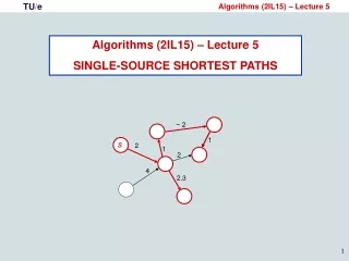
Algorithms (2IL15) – Lecture 5 SINGLE-SOURCE SHORTEST PATHS − 2 1 s 2 1 2 4 2.3
− 2 1 2 1 2 2.3 4 4 3 1 5 3 2 8 3 Part II of the course: optimization problems on graphs single-source shortest paths Find shortest path from source vertex to all other vertices all-pairs shortest paths Find shortest paths between all pairs of vertices maximum flow Find maximum flow from source vertex to target vertex maximum bipartite matching Find maximum number of disjoint pairs of vertices with edge between them
weighted, directed graph v4 Graph terminology graph G = (V,E ) • V = set of vertices (or: nodes) • E = set of edges (or: arcs) • (edge-)weighted graph: every edge (u,v) has a weight w(u,v) • directed graph vs. undirected graph • paths and cycles − 2 v3 1 v1 1 2 v5 2 v6 4 2.3 v2 v7
weighted, directed graph 1 2 3 4 5 6 7 1 2 3 4 5 6 7 v4 Representation of graphs, I − 2 v3 1 v1 1 2 v5 2 v6 4 2.3 v2 v7 adjacency-matrix representation M [ i,j ] = 0 if i = j w(vi,vj)if i ≠ j and edge (vi,vj) exists; w(vi,vj) is weight of (vi,vj) if edge (vi,vj) does not exist 8
4 6 -2 2 6 4 3 5 2 1 weighted, directed graph v4 Representation of graphs, II − 2 v3 1 v1 2 1 5 1 v5 2 v6 4 2.3 7 2.3 v2 v7 adjacency-list representation there is an edge from v1 to v6with weight 2 today we assume adjacency-list representation
weighted, directed graph v4 Shortest paths weighted, directed graph G = (V,E ) • weight (or: length) of a path = sum of edge weights • δ (u,v) = distance from u to v = min weight of any path from u to v • shortest path from u to v = any path from u to v of weight δ (u,v) − 2 v3 1 v1 2 1 v5 2 v6 4 2.3 v2 v7 weight = 4 weight = 2 δ(v1,v5) = 2 Is δ (u,v) always well defined? No, not if there are negative-weight cycles. If δ (u,v) well defined, then there is a shortest path with at most |V |−1 edges
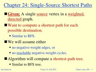
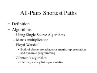
Shortest-paths problem single-pair find shortest path for single pair u,v of vertices can be solved using single-source problem with source = u and no better solutions are known single-source find shortest path from given source to all other vertices this week single-destination find shortest paths to given destination from all other vertices same as single-source for undirected graphs, for directed graphs just reverse edge directions all-pairs find shortest paths between all pairs of vertices can be solved by running single-source for each vertex, but better solutions are known: next week
v4 The Single-Source Shortest-Paths Problem Input: • graph G = (V,E) • source vertex s V output • for each v V: distanceδ (s,v) store distance in attribute d(v) if v not reachable: δ (s,v) = • a shortest-path tree that encodes all shortest paths from s: for v ≠ s thepredecessorπ(v)on a shortest path from s to v − 2 v3 s 1 v1 2 1 v5 2 v6 4 2.3 8 v2 v7 d(v2) = π(v2) = NIL 8 d(v7) = 4.3 π(v7) = v6 book (3rd ed) uses v.d and v.π instead of d(v) and π(v) NB if negative-weight cycle is reachable from s, then we only need to report this fact
2 2 running time: Θ ( |V| + |E| ) The SSSP problem on unweighted graphs Breadth-First Search (BFS) 1 0 s 1 2 1 2 1 1 2 round i: for each vertex u at distance i-1 from s ( that is, with d(v)=i-1 ) do for all neighbors v of u do if v unvisited then set d(v)=i implementation: maintain queue Q initial part of Q: nodes with d(v)=i-1 that have not been handled yet rest of Q: nodes with d(v)=i with a neighbor that has been handled
The SSSP problemon weighted graphs Dijkstra’s algorithm • works only for non-negative edge weights • running time Θ ( |V| log |V| + |E| ) Bellman-Ford algorithm • can handle negative edge weights, works even for negative-weight cycles • running time Θ ( |V| ∙ |E| ) Special case: directed acyclic graph (DAG) • can handle negative edge weights • running time Θ ( |V| + |E| )
Framework for solving SSSP problems For each vertex v, maintain value d(v) that is current “estimate” of δ (s,v) and pointer π(v) to predecessor in current shortest-path tree • Invariant: d(v) ≥ δ (s,v) if d(v) < : there exists s-to-v path of weight d(v) in which π(v) is predecessor of v • at end of algorithm: d(v) = δ (s,v) and so pointers π(v) encode shortest-path tree 8 Initialize-Single-Source (G,s) 1. for each vertex v dod(v) ← d(s) ← 0 ; π(v) ← NIL 8
8 (if d(u) = then nothing happens) Framework for solving SSSP problems For each vertex v, maintain value d(v) that is current “estimate” of δ (s,v) and pointer π(v) to predecessor in current shortest-path tree • Invariant: d(v) ≥ δ (s,v) if d(v) < : there exists s-to-v path of weight d(v) in which π(v) is predecessor of v • at end of algorithm: d(v) = δ (s,v) and so pointers π(v) encode shortest-path tree Estimates d(v) are updated using relaxation: 8 Relax( u,v ) // (u,v) is an edge ifd(u) + w(u,v) < d(v) thend(v) ← d(u) + w(u,v) 5 u v d(u)=10 d(v)=17 π(v) ← u 15
All algorithms we discuss today use this framework • algorithms differ in how they determine which edge to relax next • NB: a single edge can be relaxed multiple times Lemma (path-relaxation property): Let s,v1,v2,…,vk be a shortest path. Suppose we relax the edges of the path in order, with possibly other relax-operations in between: …, Relax(s,v1), …, Relax(v1,v2), … , Relax(v2,v3), …. , …, …, Relax(vk-1,vk), … Then after these relax-operations we have d(vk) = δ (s,vk). Proof: Induction on k. Recall that we always have d(vk) ≥ δ (s,vk). • base case, k=1: after Relax(s,v1) we have d(v1) ≤ d(s) + w(s,v1) = δ (s,v1) • k >1: just before Relax(vk-1,vk) we have d(vk-1) = δ (s,vk-1) by induction. after Relax(vk-1,vk) we thus have d(vk) ≤ d(vk-1) + w(vk-1,vk) = δ (s,vk-1) + w(vk-1,vk) = δ (s,vk)
Dijkstra’s algorithm • Input: • weighted graph G(V,E) with non-negative edge weights • source node s • Required output: • for each vertex v: • value d(v) = δ(s,v) • pointer π(v) to parent in shortest-path tree
2 2 1 Let’s see if we can adapt BFS 0 s 1 2 1 2 1 1 2 round i: for each vertex u at distance i-1 from s ( that is, with d(v)=i-1 ) dofor all neighbors v of u do if v unvisited then set d(v)=i when edges have weights, distances can “jump” and we cannot handle vertices in rounds as in BFS … … but we can still try to handle vertices in order of increasing distance to s this is a Relax-operation
s s Dijkstra’s algorithm • handle vertices in increasing distance to s • handling a vertex = relax all outgoing edges 3 4 4 8 8 1 relax 4 3 relax relax 1 relax 1 relax relax relax d(s) = 0 2 4 8 8 6 2 5 • Implementation:maintain priority queue Q • Q contains vertices that have not been handled yet; key = d(v)
Dijkstra (G,s) // G = (V,E) is a weighted directed graph with no negative edge weights • Initialize-Single-Source ( G,s ) • S ← empty set // S = set of vertices that have been handled • Put all vertices v in V in min-priority queue Q, with d(v) as key • whileQ not empty • dou ← Extract-Min(Q) • S ← S U { u } • for each outgoing edge (u,v) • do Relax(u,v) if d(v) changes, we have to update Q: Relax( u,v ) // (u,v) is an edge ifd(u) + w(u,v) < d(v) thend(v) ← d(u) + w(u,v) π(v) ← u Decrease-Key (Q, v, d(v) ) change key of v to (new, lower value of) d(v)
Dijkstra (G,s) // G = (V,E) is a weighted directed graph with no negative edge weights • Initialize-Single-Source ( G,s ) • S ← empty set // S = set of vertices that have been handled • Put all vertices v in V in min-priority queue Q, with d(v) as key • whileQ not empty • dou ← Extract-Min(Q) • S ← S U { u } • for each outgoing edge (u,v) • do Relax(u,v) Invariant: at start of each iteration of while-loop: d(v) = δ(s,v) for all v in S. Intialization:S ← empty set, so Invariant holds before first iteration
Invariant: at start of each iteration of while-loop: d(v) = δ(s,v) for all v in S. Maintenance: must prove d(u) = δ(s,u) for selected vertex u x y u s first vertex on shortest path to u that has not yet been handled no negative edge-weights x has been handled (x,y) has been relaxed d(y) = δ(s,y) u was chosen if y = u: okay otherwise: d(u) ≤ d(y) = δ(s,y) ≤ δ(s,u) d(u) ≥ δ(s,u) by property of Relax d(u) = δ(s,u)
Invariant: at start of each iteration of while-loop: d(v) = δ(s,v) for all v in S. Termination: • initially Q contains |V | vertices at every iteration size of Q decreases by one • at end of algorithm: Q is empty we always have Q = V − S Invariant: d(v) = δ(s,v) for all v in S termination after |V| iterations algorithm is correct
Dijkstra (G,s) // G = (V,E) is a weighted directed graph with no negative edge weights • Initialize-Single-Source ( G,s ) • S ← empty set // S = set of vertices that have been handled • Put all vertices v in V in min-priority queue Q, with d(v) as key • whileQ not empty • dou ← Extract-Min(Q) • S ← S U { u } • for each outgoing edge (u,v) • do Relax(u,v) Running time: • number of Extract-Min operations = • number of Relax-operations = Relax involves Decrease-Key-operation normal heap: Extract-Min and Decrease-Key both O(log n) Fibonacci heap: Extract-Min O(log n), Decrease-Key O(1) on average |V| |E| O( (V+E) log V ) O( V log V + E )
Theorem: Dijkstra’s algorithm solves the Single-Source Shortest-Path Problem for graphs with non-negative edge weights in O( |V| log |V| + |E| ) time.
Bellman-Ford algorithm • Input: • weighted graph G(V,E), can havenegative edge weights • source node s • Required output: • for each vertex v: • value d(v) = δ(s,v) • pointer π(v) to parent in shortest-path tree • or report there is a negative-weight cycle reachable from s
Recall path-relaxation property Lemma: Let s,v1,v2,…,vk be a shortest path. Suppose we relax the edges of the path in order, with possibly other relax-operations in between: …, Relax(s,v1), …, Relax(v1,v2), … , Relax(v2,v3), …. , …, …, Relax(vk-1,vk), … Then after these relax-operations we have d(vk) = δ (s,vk). Problem with negative weights: we don’t know in which order to relax edges Idea of Bellman-Ford algorithm • after relaxing all edges we have relaxed the first edge on any shortest path • after relaxing all edges once more, we have relaxed the second edge • etc.
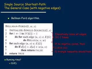
Bellman-Ford (G,s) // G = (V,E) is a weighted directed graph; edge weights may be negative • Initialize-Single-Source ( G,s ) • for i ← 1 to |V | − 1 • dofor each edge (u,v) in E • do Relax(u,v) // Check for negative length cycles: • for each edge (u,v) in E • doifd(u) + w(u,v) < d(v) // there is an edge that could still be relaxed • then report there is a negative-weight cycle reachable from s −1 0 8 8 w(e1)=1 w(e2)=−3 w(e3)=1 s d(s) = 0 w(e4)=2 w(e5)=4 8 8 2 1
Bellman-Ford (G,s) // G = (V,E) is a weighted directed graph; edge weights may be negative • Initialize-Single-Source ( G,s ) • for i ← 1 to |V | − 1 • dofor each edge (u,v) in E • do Relax(u,v) // Check for negative length cycles: • for each edge (u,v) in E • doifd(u) + w(u,v) < d(v) // there is an edge that could still be relaxed • then report there is a negative-weight cycle reachable from s Correctness, in case of no reachable negative-weight cycles: Invariant of the loop in lines 2 – 4 (follows from path-relaxation property): for each v with shortest path from s consisting of ≤i edges, we have d(v) = δ(s,v) So after the loop, we have: d(v) = δ(s,v) for all v in V and algorithm will not report a negative-weight cycle in line 7
+ Correctness in case of reachable negative-weight cycle: v1,v2,…,vk,v1: reachable negative-weight cycle Assume for contradiction that d(vi) + w(vi,vi+1) ≥ d(vi+1) for all i=1,…,k Then: d(v1) + w(v1,v2) ≥ d(v2) d(v2) + w(v2,v3) ≥ d(v3) … d(vk-1) + w(vk-1,vk) ≥ d(vk) d(vk) + w(vk,v1) ≥ d(v1) ∑1≤i≤k d(vi) + ( ∑1≤i≤k w(vi,vi+1) + w(vk,v1) ) ≥ ∑1≤i≤k d(vi) So ∑1≤i≤k w(vi,vi+1) + w(vk,v1) ≥ 0, contradicting that cycle has negative weight.
Bellman-Ford (G,s) // G = (V,E) is a weighted directed graph; edge weights may be negative • Initialize-Single-Source ( G,s ) • for i ← 1 to |V | − 1 • dofor each edge (u,v) in E • do Relax(u,v) // Check for negative length cycles: • for each edge (u,v) in E • doifd(u) + w(u,v) < d(v) // there is an edge that could still be relaxed • then report there is a negative-weight cycle reachable from s Running time: O( |V | ∙ |E| )
Theorem: The Bellman-Ford algorithm solves the Single-Source Shortest-Path Problem (even in case of negative-weight cycles) in O( |V | ∙ |E| ) time.
The SSSP problemon weighted graphs: summary Bellman-Ford algorithm • can handle negative edge weights, works even for negative-weight cycles • running time Θ ( |V | ∙ |E| ) Dijkstra’s algorithm • works only for non-negative edge weights • running time Θ ( |V | log |V | + |E| ) Special case: directed acyclic graph (DAG): see the book • can handle negative edge weights • running time Θ ( |V | + |E| ) Next week: the All-Pairs Shortest-Path Problem