Shortest Paths
Shortest Paths. Definitions Single Source Algorithms Bellman Ford DAG shortest path algorithm Dijkstra All Pairs Algorithms Using Single Source Algorithms Matrix multiplication Floyd-Warshall Both of above use adjacency matrix representation and dynamic programming Johnson’s algorithm

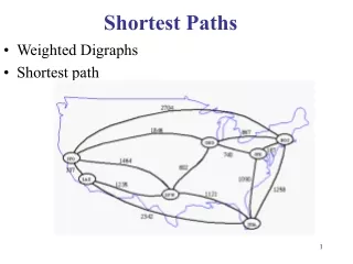
Shortest Paths
E N D
Presentation Transcript
Shortest Paths • Definitions • Single Source Algorithms • Bellman Ford • DAG shortest path algorithm • Dijkstra • All Pairs Algorithms • Using Single Source Algorithms • Matrix multiplication • Floyd-Warshall • Both of above use adjacency matrix representation and dynamic programming • Johnson’s algorithm • Uses adjacency list representation
Single Source Definition • Input • Weighted, connected directed graph G=(V,E) • Weight (length) function w on each edge e in E • Source node s in V • Task • Compute a shortest path from s to all nodes in V
All Pairs Definition • Input • Weighted, connected directed graph G=(V,E) • Weight (length) function w on each edge e in E • We will typically assume w is represented as a matrix • Task • Compute a shortest path from all nodes in V to all nodes in V
Comments • If edges are not weighted, then BFS works for single source problem • Optimal substructure • A shortest path between s and t contains other shortest paths within it • No known algorithm is better at finding a shortest path from s to a specific destination node t in G than finding the shortest path from s to all nodes in V
Negative weight edges • Negative weight edges can be allowed as long as there are no negative weight cycles • If there are negative weight cycles, then there cannot be a shortest path from s to any node t (why?) • If we disallow negative weight cycles, then there always is a shortest path that contains no cycles
Relaxation technique • For each vertex v, we maintain an upper bound d[v] on the length of shortest path from s to v • d[v] initialized to infinity • Relaxing an edge (u,v) • Can we shorten the path to v by going through u? • If d[v] > d[u] + w(u,v), d[v] = d[u] + w(u,v) • This can be done in O(1) time
Bellman-Ford (G, w, s) Initialize-Single-Source(G,s) for (i=1 to V-1) for each edge (u,v) in E relax(u,v); for each edge (u,v) in E if d[v] > d[u] + w(u,v) return NEGATIVE WEIGHT CYCLE -5 -5 3 3 5 5 -1 7 s s 1 1 3 3 2 2 Bellman-Ford Algorithm G1 G2
Running Time • for (i=1 to V-1) • for each edge (u,v) in E • relax(u,v); • The above takes (V-1)O(E) = O(VE) time • for each edge (u,v) in E • if d[v] > d[u] + w(u,v) • return NEGATIVE WEIGHT CYCLE • The above takes O(E) time
Proof of Correctness • Theorem: If there is a shortest path from s to any node v, then d[v] will have this weight at end of Bellman-Ford algorithm • Theorem restated: • Define links[v] to be the minimum number of edges on a shortest path from s to v • After i iterations of the Bellman-Ford for loop, nodes v with links[v] ≤ i will have their d[v] value set correctly • Prove this by induction on links[v] • Base case: links[v] = 0 which means v is s • d[s] is initialized to 0 which is correct unless there is a negative weight cycle from s to s in which case there is no shortest path from s to s. • Induction hypothesis: After k iterations for k ≥ 0, d[v] must be correct if links[v] ≤ k • Inductive step: Show after k+1 iterations, d[v] must be correct if links[v] ≤ k+1 • If links[v] ≤ k, then by IH, d[v] is correctly set after kth iteration • If links[v] = k+1, let p = (e1, e2, …, ek+1) = (v0, v1, v2, …, vk+1) be a shortest path from s to v • s = v0, v = vk+1, ei = (vi-1, vi) • In order for links[v] = k+1, then links[vk] = k. • By the inductive hypothesis, d[vk] will be correctly set after the kth iteration. • During the k+1st iteration, we relax all edges including edge ek+1 = (vk,v) • Thus, at end of the k+1st iteration, d[v] will be correct
Negative weight cycle • for each edge (u,v) in E • if d[v] > d[u] + w(u,v) • return NEGATIVE WEIGHT CYCLE • If no neg weight cycle, d[v] ≤d[u] + w(u,v) for all (u,v) • If there is a negative weight cycle C, for some edge (u,v) on C, it must be the case that d[v] > d[u] + w(u,v). • Suppose this is not true for some neg. weight cycle C • sum these (d[v] ≤ d[u] + w(u,v)) all the way around C • We end up with Σv in C d[v] ≤ (Σu in C d[u]) + weight(C) • This is impossible unless weight(C) = 0 • But weight(C) is negative, so this cannot happen • Thus for some (u,v) on C, d[v] > d[u] + w(u,v)
DAG-SP (G, w, s) Initialize-Single-Source(G,s) Topologically sort vertices in G for each vertex u, taken in sorted order for each edge (u,v) in E relax(u,v); DAG shortest path algorithm 5 3 4 -4 s 5 1 3 8
Running time Improvement • O(V+E) for the topological sorting • We only do 1 relaxation for each edge: O(E) time • for each vertex u, taken in sorted order • for each edge (u,v) in E • relax(u,v); • Overall running time: O(V+E)
Proof of Correctness • If there is a shortest path from s to any node v, then d[v] will have this weight at end • Let p = (e1, e2, …, ek) = (v1, v2, v3, …, vk+1) be a shortest path from s to v • s = v1, v = vk+1, ei = (vi, vi+1) • Since we sort edges in topological order, we will process node vi (and edge ei) before processing later edges in the path.
Dijkstra (G, w, s) /* Assumption: all edge weights non-negative */ Initialize-Single-Source(G,s) Completed = {}; ToBeCompleted = V; While ToBeCompleted is not empty u =EXTRACT-MIN(ToBeCompleted); Completed += {u}; for each edge (u,v) relax(u,v); 4 15 5 7 s 1 3 2 Dijkstra’s Algorithm
Running Time Analysis • While ToBeCompleted is not empty • u =EXTRACT-MIN(ToBeCompleted); • Completed += {u}; • for each edge (u,v) relax(u,v); • Each edge relaxed at most once: O(E) • Need to decrease-key potentially once per edge • Need to extract-min once per node • The node’s d[v] is then complete
Running Time Analysis cont’d • Priority Queue operations • O(E) decrease key operations • O(V) extract-min operations • Three implementations of priority queues • Array: O(V2) time • decrease-key is O(1) and extract-min is O(V) • Binary heap: O(E log V) time assuming E ≥ V • decrease-key and extract-min are O(log V) • Fibonacci heap: O(V log V + E) time • decrease-key is O(1) amortized and extract-min is O(log V)
Compare Dijkstra’s algorithm to Prim’s algorithm for MST • Dijsktra • Priority Queue operations • O(E) decrease key operations • O(V) extract-min operations • Prim • Priority Queue operations • O(E) decrease-key operations • O(V) extract-min operations • Is this a coincidence or is there something more here?
s u v Only nodes in S Proof of Correctness • Assume that Dijkstra’s algorithm fails to compute length of all shortest paths from s • Let v be the first node whose shortest path length is computed incorrectly • Let S be the set of nodes whose shortest paths were computed correctly by Dijkstra prior to adding v to the processed set of nodes. • Dijkstra’s algorithm has used the shortest path from s to v using only nodes in S when it added v to S. • The shortest path to v must include one node not in S • Let u be the first such node.
s u v Only nodes in S Proof of Correctness • The length of the shortest path to u must be at least that of the length of the path computed to v. • Why? • The length of the path from u to v must be < 0. • Why? • No path can have negative length since all edge weights are non-negative, and thus we have a contradiction.
Computing paths (not just distance) • Maintain for each node v a predecessor node p(v) • p(v) is initialized to be null • Whenever an edge (u,v) is relaxed such that d(v) improves, then p(v) can be set to be u • Paths can be generated from this data structure
All pairs algorithms using single source algorithms • Call a single source algorithm from each vertex s in V • O(V X) where X is the running time of the given algorithm • Dijkstra linear array: O(V3) • Dijkstra binary heap: O(VE log V) • Dijkstra Fibonacci heap: O(V2 log V + VE) • Bellman-Ford: O(V2 E) (negative weight edges)
Two adjacency matrix based algorithms • Matrix-multiplication based algorithm • Let Lm(i,j) denote the length of the shortest path from node i to node j using at most m edges • What is our desired result in terms of Lm(i,j)? • What is a recurrence relation for Lm(i,j)? • Floyd-Warshall algorithm • Let Lk(i,j) denote the length of the shortest path from node i to node j using only nodes within {1, …, k} as internal nodes. • What is our desired result in terms of Lk(i,j)? • What is a recurrence relation for Lk(i,j)?
Shortest path using at most 2m edges Try all possible nodes k i k j Shortest path using at most m edges Shortest path using at most m edges Shortest path using nodes 1 through k i j Shortest path using nodes 1 through k-1 Shortest path using nodes 1 through k-1 Conceptual pictures Shortest path using nodes 1 through k-1 k OR
Running Times • Matrix-multiplication based algorithm • O(V3 log V) • log V executions of “matrix-matrix” multiplication • Not quite matrix-matrix multiplication but same running time • Floyd-Warshall algorithm • O(V3) • V iterations of an O(V2) update loop • The constant is very small, so this is a “fast” O(V3)
Johnson’s Algorithm • Key ideas • Reweight edge weights to eliminate negative weight edges AND preserve shortest paths • Use Bellman-Ford and Dijkstra’s algorithms as subroutines • Running time: O(V2 log V + VE) • Better than earlier algorithms for sparse graphs
Reweighting • Original edge weight is w(u,v) • New edge weight: • w’(u,v) = w(u,v) + h(u) – h(v) • h(v) is a function mapping vertices to real numbers • Key observation: • Let p be any path from node u to node v • w’(p) = w(p) + h(u) – h(v)
-5 3 4 7 1 3 -7 Computing vertex weights h(v) • Create a new graph G’ = (V’, E’) by • adding a new vertex s to V • adding edges (s,v) for all v in V with w(s,v) = 0 • Set h(v) to be the length of the shortest path from this new node s to node v • This is well-defined if G’ does not contain negative weight cycles • Note that h(v) ≤ h(u) + w(u,v) for all (u,v) in E’ • Thus, w’(u,v) = w(u,v) + h(u) – h(v) ≥ 0
Algorithm implementation • Run Bellman-Ford on G’ from new node s • If no negative weight cycle, then use h(v) values from Bellman-Ford • Now compute w’(u,v) for each edge (u,v) in E • Now run Dijkstra’s algorithm using w’ • Use each node as source node • Modify d[u,v] at end by adding h(v) and subtracting h(u) to get true path weight • Running time: • O(VE) [from one run of Bellman-Ford] + • O(V2 log V + VE) [from V runs of Dijkstra]