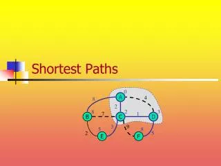
Shortest paths
Shortest paths. Given: A single source vertex (given s) in a weighted , directed graph. Want to compute a shortest path for each possible destination. ( Single Source Shortest Paths ) SSSP. Similar to BFS. We will assume either no negative-weight edges, or

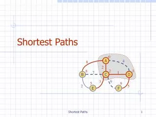
Shortest paths
E N D
Presentation Transcript
Shortest paths • Given: A single source vertex (given s) in a weighted, directed graph. • Want to compute a shortest path for each possible destination. • (Single Source Shortest Paths) SSSP. • Similar to BFS. • We will assume either • no negative-weight edges, or • no reachable negative-weight cycles. • Algorithms • Dijkstra’s (in comparison to MST prim) • Bellman-Ford • DAG Shortest Paths • The shortest paths between all pairs of vertices (All Pairs Shortest Paths). Floyd Warshall Algorithm (DP), Johnson’s. • where the length of a path is the sum of its edge weights.
props • Triangle inequality (Lemma 24.10) • For any edge (u, v) ²E, we have δ(s, v) ≤ δ(s, u) + w(u, v). • Upper-bound property (Lemma 24.11) • We always have d[v] ≥ δ(s, v) for all vertices v ²V, and once d[v] achieves • the value δ(s, v), it never changes. • No-path property (Corollary 24.12) • If there is no path from s to v, then we always have d[v] = δ(s, v)=∞. • Convergence property (Lemma 24.14) • If s ❀ u → v is a shortest path in G for some u, v ∈ V, and if d[u] = δ(s, u) at • any time prior to relaxing edge (u, v), then d[v] = δ(s, v) at all times afterward. • Path-relaxation property (Lemma 24.15) • If p = v0, v1, . . . , vk is a shortest path from s = v0 to vk , and the edges of p • are relaxed in the order (v0, v1), (v1, v2), . . . , (vk−1, vk ), then d[vk ] = δ(s, vk ). • This property holds regardless of any other relaxation steps that occur, even if • they are intermixed with relaxations of the edges of p. • Predecessor-subgraph property (Lemma 24.17) • Once d[v] = δ(s, v) for all v ∈ V, the predecessor subgraph, p[u] is a shortest-paths.
A Fact About Shortest Paths • Theorem: If p is a shortest path from u to v, then any subpath of p is also a shortest path. • Proof: Consider a subpath of p from x to y. If there were a shorter path from x to y, then there would be a shorter path from u to v. shorter? u x y v
Single-Source Shortest Paths • Given a directed graph with weighted edges, what are the shortest paths from some source vertex s to all other vertices? • Note: shortest path to single destination cannot be done asymptotically faster, as far as we know. 6 3 9 3 2 4 0 1 7 2 s 3 5 5 11 6
u v u v 6 3 9 6 3 9 3 s 3 2 4 s 0 2 2 1 7 4 0 3 1 3 2 7 5 5 5 11 5 11 6 6 x x y y Path Recovery • We would like to find the path itself, not just its length. We’ll construct a shortest-paths tree:
Shortest-Paths Idea • d(u,v) length of the shortest path from u to v. • All SSSP algorithms maintain a field d[u] for every vertex u. d[u] will be an estimate ofd(s,u). As the algorithm progresses, we will refine d[u] until, at termination, d[u] = d(s,u). Whenever we discover a new shortest path to u, we update d[u]. • In fact, d[u] will always be an overestimate of d(s,u): • d[u] ³ d(s,u) • We’ll use p[u] to point to the parent (or predecessor) of u on the shortest path from s to u. We update p[u] when we update d[u].
SSSP Subroutine RELAX(u, v, w) > (Maybe) improve our estimate of the distance to v > by considering a path along the edge (u, v). if d[u] + w(u, v) < d[v] then d[v] ¬ d[u] + w(u, v)> actually, DECREASE-KEY p[v] ¬ u > remember predecessor on path d[u] d[v] w(u,v) u v
Shortest Path Properties • Again, we have optimal substructure: the shortest path consists of shortest subpaths: • Proof: suppose some subpath is not a shortest path • There must then exist a shorter subpath • Could substitute the shorter subpath for a shorter path • But then overall path is not shortest path. Contradiction
Shortest Path Properties • Define (u,v) to be the weight of the shortest path from u to v • Shortest paths satisfy the triangle inequality: (u,v) (u,x) + (x,v) • “Proof”: x u v This path is no longer than any other path
Shortest Path Properties • In graphs with negative weight cycles, some shortest paths will not exist (Why?): < 0
2 2 9 6 5 5 Relax Relax 2 2 7 6 5 5 Relaxation • A key technique in shortest path algorithms is relaxation • Idea: for all v, maintain upper bound d[v] on (s,v) Relax(u,v,w) { if (d[v] > d[u]+w) then d[v]=d[u]+w; }
Dijkstra’s Algorithm • (pronounced “DIKE-stra”) • Assume that all edge weights are 0. • Idea: say we have a set K containing all vertices whose shortest paths from s are known (i.e. d[u] = d(s,u) for all u in K). • Now look at the “frontier” of K—all vertices adjacent to a vertex in K. the rest of the graph K s
Dijkstra’s: Theorem • At each frontier vertex u, update d[u] to be the minimum from all edges from K. • Now pick the frontier vertex u with the smallest value of d[u]. • Claim: d[u] = d(s,u) min(4+2, 6+1) = 6 2 4 6 1 8 s 6 9 3 min(4+8, 6+3) = 9
Dijkstra’s: Proof • By construction, d[u]is the length of the shortest path to u going through only vertices in K. • Another path to u must leave K and go to v on the frontier. • But the length of this path is at least d[v], (assuming non-negative edge weights), which is ³d[u].
u s v Proof Explained • Why is the path through v at least d[v] in length? • We know the shortest paths to every vertex in K. • We’ve set d[v] to the shortest distance from s to v via K. • The additional edges from v to u cannot decrease the path length. shortest path to u d[u] £ d[v] K another path to u, via v
A Refinement • Note: we don’t really need to keep track of the frontier. • When we add a new vertex u to K, just update vertices adjacent to u.
Dijkstra Running Time (cont.) • 1. Priority queue is an array.EXTRACT-MIN in (n) time, DECREASE-KEY in (1)Total time: (V + VV + E) = (V2) • 2. (“Modified Dijkstra”)Priority queue is a binary (standard) heap.EXTRACT-MIN in (lgn) time, also DECREASE-KEYTotal time: (VlgV + ElgV) • 3. Priority queue is Fibonacci heap. (Of theoretical interest only.)EXTRACT-MIN in (lgn), DECREASE-KEY in (1) (amortized)Total time: (VlgV+E)
The Bellman-Ford Algorithm • Handles negative edge weights • Detects negative cycles • Is slower than Dijkstra 4 -10 5 a negative cycle
Bellman-Ford: Idea • Repeatedly update d for all pairs of vertices connected by an edge. • Theorem: If u and v are two vertices with an edge from u to v, and s u v is a shortest path, and d[u] = d(s,u), • then d[u]+w(u,v) is the length of a shortest path to v. • Proof: Since s u v is a shortest path, its length is d(s,u) + w(u,v) = d[u] + w(u,v).
Why Bellman-Ford Works • On the first pass, we find d (s,u) for all vertices whose shortest paths have one edge. • On the second pass, the d[u] values computed for the one-edge-away vertices are correct (= d (s,u)), so they are used to compute the correct d values for vertices whose shortest paths have two edges. • Since no shortest path can have more than |V[G]|-1 edges, after that many passes all d values are correct. • Note: all vertices not reachable from s will have their original values of infinity. (Same, by the way, for Dijkstra).
Bellman-Ford: Algorithm • BELLMAN-FORD(G, w, s) • 1 foreach vertex v ÎV[G] do //INIT_SINGLE_SOURCE • 2 d[v] ¬ ¥ • 3 p[v] ¬ NIL • 4 d[s] ¬ 0 • 5 for i ¬ 1 to |V[G]|-1 do >each iteration is a “pass” • 6 for each edge (u,v) in E[G] do • 7 RELAX(u, v, w) • 8 >check for negative cycles • 9 for each edge (u,v) in E[G] do • 10 if d[v] > d[u] + w(u,v) then • 11 return FALSE • 12 return TRUE Running time: Q(VE)
Negative Cycle Detection • What if there is a negative-weightcycle reachable from s? • Assume: d[u] £ d[x]+4 • d[v] £ d[u]+5 • d[x] £ d[v]-10 • Adding: • d[u]+d[v]+d[x] £ d[x]+d[u]+d[v]-1 • Because it’s a cycle, vertices on left are same as those on right. Thus we get 0 £ -1; a contradiction. So for at least one edge (u,v), • d[v] > d[u] + w(u,v) • This is exactly what Bellman-Ford checks for. x 4 u -10 v 5
Example u v 5 –2 6 –3 8 0 z 7 –4 2 7 9 y x
Example u v 5 6 –2 6 –3 8 0 z 7 –4 2 7 7 9 y x
Example u v 5 6 4 –2 6 –3 8 0 z 7 –4 2 7 2 7 9 y x
Example u v 5 2 4 –2 6 –3 8 0 z 7 –4 2 7 2 7 9 y x
Example u v 5 2 4 –2 6 –3 8 0 z 7 –4 2 7 -2 7 9 y x
BF Dynamic aspect for the same graph Note: This is essentially dynamic programming. Let d(i, j) = cost of the shortest path from s to i that is at most j hops. d(i, j) = 0 if i = s j = 0 if i s j = 0 min({d(k, j–1) + w(k, i): i Adj(k)} {d(i, j–1)}) if j > 0 i z u v x y 1 2 3 4 5 0 0 1 0 6 7 2 0 6 4 7 2 3 0 2 4 7 2 4 0 2 4 7 –2 j
Bellman-Ford where G contains no negative weight cycles(iterations from E to A) π: nil d: 0 π: nil d: ∞ 2 A B -1 π: nil d: ∞ 2 3 -3 C 4 5 3 -1 D E 4 π: nil d: ∞ π: nil d: ∞
π: nil d: 0 π: nil A d: ∞ -1 2 A B -1 π: nil C d: ∞ 2 2 3 -3 C 4 5 3 -1 D E 4 π: nil A d: ∞ 4 π: nil d: ∞
π: nil d: 0 π: nil A d: ∞ -1 2 A B -1 π: nil C d: ∞ 2 2 3 -3 C 4 5 3 -1 D E 4 π: nil A d: ∞ 4 π: nil C d: ∞ 3
π: nil d: 0 π: nil A d: ∞ -1 2 A B -1 π: nil C d: ∞ 2 2 3 -3 C 4 5 3 -1 D E 4 π: nil A d: ∞ 4 π: nil C d: ∞ 3
π: nil d: 0 π: nil A d: ∞ -1 2 A B -1 π: nil C d: ∞ 2 2 3 -3 C 4 5 3 -1 D E 4 π: nil A d: ∞ 4 π: nil C d: ∞ 3
Bellman-Ford where G contains no negative weight cycles(iterations from A to E) π: nil d: 0 π: nil d: ∞ 2 A B -1 π: nil d: ∞ 2 1 -3 C 4 5 1 -1 D E 4 π: nil d: ∞ π: nil d: ∞
π: nil d: 0 π: nil A d: ∞ -1 2 A B -1 π: nil C d: ∞ 2 2 1 -3 C 4 5 1 -1 D E 4 π: nil A d: ∞ 4 π: nil d: ∞
π: nil d: 0 π: nil A d: ∞ -1 2 A B -1 π: nil C B d: ∞ 2 0 2 1 -3 C 4 5 1 -1 D E 4 π: nil A d: ∞ 4 π: nil C d: ∞ 3
π: nil d: 0 π: nil A d: ∞ -1 2 A B -1 π: nil C B d: ∞ 2 0 2 1 -3 C 4 5 1 -1 D E 4 π: nil A d: ∞ 4 π: nil C C d: ∞ 3 1
π: nil d: 0 π: nil A E d: ∞ -1 -2 2 A B -1 π: nil C B B d: ∞ 2 0 -1 2 1 -3 C 4 5 1 -1 D E 4 π: nil A d: ∞ 4 π: nil C C d: ∞ 3 1
Lemma 24.2 Lemma 24.2: Assuming no negative-weight cycles reachable from s, d[v] = (s, v) holds upon termination for all vertices v reachable from s. • Proof: • Consider a SP p, where p = ‹v0, v1, …, vk›, where v0 = s and vk = v. • Assume k |V| – 1, otherwise p has a cycle. • Claim: d[vi] = (s, vi) holds after the ith pass over edges. • Proof follows by induction on i. • By Lemma 24.11, once d[vi] = (s, vi) holds, it continues to hold. Comp 122, Fall 2003 Single-source SPs - 40
Correctness • Claim: Algorithm returns the correct value. • (Part of Theorem 24.4. Other parts of the theorem follow easily from earlier results.) • Case 1: There is no reachable negative-weight cycle. • Upon termination, we have for all (u, v): • d[v] = (s, v) , by lemma 24.2 (last slide) if v is reachable; • d[v] = (s, v) = otherwise. • (s, u) + w(u, v) , by Lemma 24.10. • = d[u] + w(u, v) • So, algorithm returns true. Comp 122, Fall 2003 Single-source SPs - 41
Case 2 • Case 2: There exists a reachable negative-weight cycle • c = ‹v0, v1, …, vk›, where v0 = vk. • We have i = 1, …, k w(vi-1, vi) < 0. (*) • Suppose algorithm returns true. Then, d[vi] d[vi-1] + w(vi-1, vi) for • i = 1, …, k. (because Relax didn’t change any d[vi] ). Thus, • i = 1, …, k d[vi] i = 1, …, k d[vi-1] + i = 1, …, k w(vi-1, vi) • But, i = 1, …, k d[vi] = i = 1, …, k d[vi-1]. • Can show no d[vi] is infinite. Hence, 0 i = 1, …, k w(vi-1, vi). • Contradicts (*). Thus, algorithm returns false. Comp 122, Fall 2003 Single-source SPs - 42
Review: Getting Dressed Underwear Socks Watch Pants Shoes Shirt • Topological-Sort() • { • 1- Run DFS • 2- When a vertex is finished, output it • 3- Vertices are output in reverse topological order • } • Time: O(V+E) Belt Tie Jacket Socks Underwear Pants Shoes Watch Shirt Belt Tie Jacket
SSSP in a DAG • Recall: a dag is a directed acyclic graph. • If we update the edges in topologically sorted order, we correctly compute the shortest paths. • Reason: the only paths to a vertex come from vertices before it in the topological sort. 9 s 0 1 4 6 1 3 2
SSSP in a DAG Theorem • Theorem: For any vertex u in a dag, if all the vertices before u in a topological sort of the dag have been updated, then d[u] = d(s,u). • Proof: By induction on the position of a vertex in the topological sort. • Base case: d[s] is initialized to 0. • Inductive case: Assume all vertices before u have been updated, and for all such vertices v, d[v]=d(s,v). (continued)
Proof, Continued • Some edge (v,u) where v is before u, must be on the shortest path to u, since there are no other paths to u. • When v was updated, we set d[u] to d[v]+w(v,u) • = d(s,v) + w(v,u) • = d(s,u)
DAG-SHORTEST-PATHS(G,w,s) 1 topologically sort the vertices of G 2 initialize d and p as in previous algorithms 3 for each vertex u in topological sort order do 4 for each vertex v in Adj[u] do 5 RELAX(u, v, w) Running time: q(V+E), same as topological sort SSSP-DAG Algorithm
Shortest Paths in DAGs Topologically sort vertices in G; Initialize(G, s); for each u in V[G] (in order) do for each v in Adj[u] do Relax(u, v, w) od od Comp 122, Fall 2003 Single-source SPs - 48
Example 6 1 u r t s v w 2 7 –2 5 –1 0 4 3 2 Comp 122, Fall 2003 Single-source SPs - 49
Example 6 1 u r t s v w 2 7 –2 5 –1 0 4 3 2 Comp 122, Fall 2003 Single-source SPs - 50