Shortest Paths
Learn about Dijkstra's Algorithm, a method for finding the shortest paths in graphs with nonnegative edge weights. Understand the workings, requirements, and pseudocode of this efficient algorithm.

Shortest Paths
E N D
Presentation Transcript
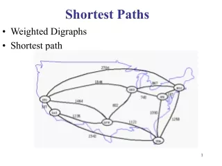
Shortest Paths • Weighted Digraphs • Shortest path
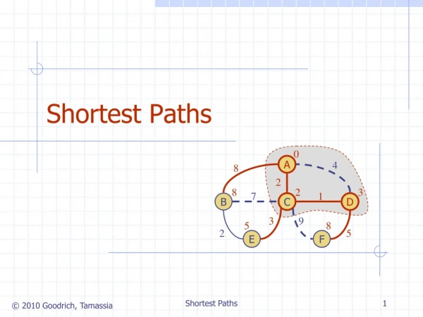
Weighted Graphs • weights on the edges of a graph represent distances, costs, etc. • An example of an undirected weighted graph:
Shortest Path • BFS finds paths with the minimum number of edges from the start vertex • Hencs, BFS finds shortest paths assuming that each edge has the same weight • In many applications, e.g., transportation networks, the edges of a graph have different weights. • How can we find paths of minimum total weight? • Example - Boston to Los Angeles:
Dijkstra’s Algorithm • Dijkstra’s algorithm finds shortest paths from a start vertex v to all the other vertices. • Requirements: it works on a graph with • undirected edges • nonnegative edge weights
Dijkstra’s Algorithm: at work • The algorithm computes for each vertex u the distance to u from the start vertex v, that is, the weight of a shortest path between v and u. • the algorithm keeps track of the set of vertices for which the distance has been computed, called the cloud C • Every vertex has a label D associated with it. For any vertex u, we can refer to its D label as D[u]. D[u] stores an approximation of the distance between v and u. The algorithm will update a D[u] value when it finds a shorter path from v to u. • When a vertex u is added to the cloud, its label D[u] is equal to the actual (final) distance between the starting vertex v and vertex u. • initially, we set - D[v] = 0 ...the distance from v to itself is 0... - D[u] = ∞ for u v ...these will change...
The Algorithm: Expanding the Cloud • Repeat until all vertices have been put in the cloud: • let u be a vertex not in the cloud that has smallest label D[u]. (On the first iteration, naturally the starting vertex will be chosen.) • we add u to the cloud C • we update the labels of the adjacent vertices of u as follows: for each vertex z adjacent tou do ifz is not in the cloud C then ifD[u] + weight(u,z) < D[z] then D[z] = D[u] + weight(u,z) • the above step is called a relaxation of edge (u,z)
Pseudocode Algorithm ShortestPath(G, v): Input: A weighted graph G and a distinguished vertex v of G. Output: A label D[u], for each vertex that u of G, such that D[u] is the length of a shortest path from v to u in G. initialize D[v] 0 and D[u] ∞ +∞ for each vertex v u let Q be a priority queue that contains all of the vertices of G using the D lables as keys. while Q do {pull u into the cloud C} u Q.removeMinElement() for each vertex z adjacent to u such that z is in Q do {perform the relaxation operation on edge (u, z) } if D[u] + w((u, z)) < D[z] then D[z] D[u] + w((u, z)) change the key value of z in Q to D[z] return the label D[u] of each vertex u. • we use a priority queue Q to store the vertices not in the cloud, where D[v] the key of a vertex v in Q
Running Time • Let’s assume that we represent G with an adjacency list. We can then step through all the vertices adjacent to u in time proportional to their number (i.e. O(j) where j in the number of vertices adjacent to u) • The priority queue Q - we have a choice: • A Heap: Implementing Q with a heap allows for efficient extraction of vertices with the smallest D label (Takes O(logN) time). If Q is implemented with locators, key updates can be performed in O(logN) time. The total run time is O((n+m)logn) where n is the number of vertices in G and m in the number of edges. In terms of n, worst case time is O(n2logn) • An Unsorted Sequence: O(n) when we extract minimum elements, but fast key updates (O(1)). There are only n-1 extractions and m relaxations. The running time is O(n2+m) • In terms of worst case time, heap is good for small data sets and sequence for larger.
Running Time (cont) • The average case is a slightly different story. Consider this: -If priority queue Q is implemented with a heap, the bottleneck step is updating the key of a vertex in Q. In the worst case, we would need to perform an update for every edge in the graph. -For most graphs, though, this would not happen. Using the random neighbor-order assumption, we can observe that for each vertex, its neighbor vertices will be pulled into the cloud in essentially random order. So here are only O(logn) updates to the key of a vertex. -Under this assumption, the run time of the heap implementation is O(nlogn+m), which is always O(n2). The heap implementation is thus preferable for all but degenerate cases.
Dijkstra’s Algorithm,some things to think about... • In our example, the weight is the geographical distance. However, the weight could just as easily represent the cost or time to fly the given route. • We can easily modify Dijkstra’s algorithm for different needs, for instance: • If we just want to know the shortest path from vertex v to a single vertex u, we can stop the algorithm as soon as u is pulled into the cloud. • Or, we could have the algorithm output a tree T rooted at v such that the path in T from v to a vertex u is a shortest path from v to u. • How to keep track of weights and distances? Edges and vertices do not “know” their weights/distances. Take advantage of the fact that D[u] is the key for vertex u in the priority queue, and thus D[u] can be retrieved if we know the locator of u in Q. • Need some way of: • associating PQ locators with the vertices • storing and retrieving the edge weights • returning the final vertex distance