Graph Algorithms
Graph Algorithms. Topic Overview . Definitions and Representation Minimum Spanning Tree: Prim's Algorithm Single-Source Shortest Paths: Dijkstra's Algorithm All-Pairs Shortest Paths Transitive Closure Connected Components Algorithms for Sparse Graphs .

Graph Algorithms
E N D
Presentation Transcript
Topic Overview • Definitions and Representation • Minimum Spanning Tree: Prim's Algorithm • Single-Source Shortest Paths: Dijkstra's Algorithm • All-Pairs Shortest Paths • Transitive Closure • Connected Components • Algorithms for Sparse Graphs
Definitions and Representation • An undirected graphG is a pair (V,E), where V is a finite set of points called vertices and E is a finite set of edges. • An edge e ∈ E is an unordered pair (u,v), where u,v ∈ V. • In a directed graph, the edge e is an ordered pair (u,v). An edge (u,v) is incident from vertex u and is incident to vertex v. • A path from a vertex v to a vertex u is a sequence <v0,v1,v2,…,vk> of vertices where v0 = v, vk = u, and (vi, vi+1) ∈ E for I = 0, 1,…, k-1. • The length of a path is defined as the number of edges in the path.
Definitions and Representation a) An undirected graph and (b) a directed graph.
Definitions and Representation • An undirected graph is connected if every pair of vertices is connected by a path. • A forest is an acyclic graph, and a tree is a connected acyclic graph. • A graph that has weights associated with each edge is called a weighted graph.
Definitions and Representation • Graphs can be represented by their adjacency matrix or an edge (or vertex) list. • Adjacency matrices have a value ai,j = 1 if nodes i and j share an edge; 0 otherwise. In case of a weighted graph, ai,j = wi,j, the weight of the edge. • The adjacency list representation of a graph G = (V,E) consists of an array Adj[1..|V|] of lists. Each list Adj[v] is a list of all vertices adjacent to v. • For a grapn with n nodes, adjacency matrices take Θ(n2) space and adjacency list takes Θ(|E|) space.
Definitions and Representation An undirected graph and its adjacency matrix representation. An undirected graph and its adjacency list representation.
Minimum Spanning Tree • A spanning tree of an undirected graph G is a subgraph of G that is a tree containing all the vertices of G. • In a weighted graph, the weight of a subgraph is the sum of the weights of the edges in the subgraph. • A minimum spanning tree (MST) for a weighted undirected graph is a spanning tree with minimum weight.
Minimum Spanning Tree An undirected graph and its minimum spanning tree.
Minimum Spanning Tree: Prim's Algorithm • Prim's algorithm for finding an MST is a greedy algorithm. • Start by selecting an arbitrary vertex, include it into the current MST. • Grow the current MST by inserting into it the vertex closest to one of the vertices already in current MST.
Minimum Spanning Tree: Prim's Algorithm Prim's minimum spanning tree algorithm.
Minimum Spanning Tree: Prim's Algorithm Prim's sequential minimum spanning tree algorithm.
Prim's Algorithm: Parallel Formulation • The algorithm works in n outer iterations - it is hard to execute these iterations concurrently. • The inner loop is relatively easy to parallelize. Let p be the number of processes, and let n be the number of vertices. • The adjacency matrix is partitioned in a 1-D block fashion, with distance vector d partitioned accordingly. • In each step, a processor selects the locally closest node, followed by a global reduction to select globally closest node. • This node is inserted into MST, and the choice broadcast to all processors. • Each processor updates its part of the d vector locally.
Prim's Algorithm: Parallel Formulation The partitioning of the distance array d and the adjacency matrix A among p processes.
Prim's Algorithm: Parallel Formulation • The cost to select the minimum entry is O(n/p + log p). • The cost of a broadcast is O(log p). • The cost of local updation of the d vector is O(n/p). • The parallel time per iteration is O(n/p + log p). • The total parallel time is given by O(n2/p + n log p). • The corresponding isoefficiency is O(p2log2p).
Single-Source Shortest Paths • For a weighted graph G = (V,E,w), the single-source shortest paths problem is to find the shortest paths from a vertex v ∈ V to all other vertices in V. • Dijkstra's algorithm is similar to Prim's algorithm. It maintains a set of nodes for which the shortest paths are known. • It grows this set based on the node closest to source using one of the nodes in the current shortest path set.
Single-Source Shortest Paths: Dijkstra's Algorithm Dijkstra's sequential single-source shortest paths algorithm.
Dijkstra's Algorithm: Parallel Formulation • Very similar to the parallel formulation of Prim's algorithm for minimum spanning trees. • The weighted adjacency matrix is partitioned using the 1-D block mapping. • Each process selects, locally, the node closest to the source, followed by a global reduction to select next node. • The node is broadcast to all processors and the l-vector updated. • The parallel performance of Dijkstra's algorithm is identical to that of Prim's algorithm.
All-Pairs Shortest Paths • Given a weighted graph G(V,E,w), the all-pairs shortest paths problem is to find the shortest paths between all pairs of vertices vi, vj∈ V. • A number of algorithms are known for solving this problem.
All-Pairs Shortest Paths: Matrix-Multiplication Based Algorithm • Consider the multiplication of the weighted adjacency matrix with itself - except, in this case, we replace the multiplication operation in matrix multiplication by addition, and the addition operation by minimization. • Notice that the product of weighted adjacency matrix with itself returns a matrix that contains shortest paths of length 2 between any pair of nodes. • It follows from this argument that An contains all shortest paths.
Matrix-Multiplication Based Algorithm • An is computed by doubling powers - i.e., as A, A2, A4, A8, and so on. • We need log n matrix multiplications, each taking time O(n3). • The serial complexity of this procedure is O(n3log n). • This algorithm is not optimal, since the best known algorithms have complexity O(n3).
Matrix-Multiplication Based Algorithm: Parallel Formulation • Each of the log n matrix multiplications can be performed in parallel. • We can use n3/log n processors to compute each matrix-matrix product in time log n. • The entire process takes O(log2n) time.
Dijkstra's Algorithm • Execute n instances of the single-source shortest path problem, one for each of the n source vertices. • Complexity is O(n3).
Dijkstra's Algorithm: Parallel Formulation • Two parallelization strategies - execute each of the n shortest path problems on a different processor (source partitioned), or use a parallel formulation of the shortest path problem to increase concurrency (source parallel).
Dijkstra's Algorithm: Source Partitioned Formulation • Use n processors, each processor Pi finds the shortest paths from vertex vi to all other vertices by executing Dijkstra's sequential single-source shortest paths algorithm. • It requires no interprocess communication (provided that the adjacency matrix is replicated at all processes). • The parallel run time of this formulation is: Θ(n2). • While the algorithm is cost optimal, it can only use n processors. Therefore, the isoefficiency due to concurrency is p3.
Dijkstra's Algorithm: Source Parallel Formulation • In this case, each of the shortest path problems is further executed in parallel. We can therefore use up to n2processors. • Given p processors (p > n), each single source shortest path problem is executed by p/n processors. • Using previous results, this takes time: • For cost optimality, we have p = O(n2/log n) and the isoefficiency is Θ((p log p)1.5).
Floyd's Algorithm • For any pair of vertices vi, vj∈ V, consider all paths from vi to vj whose intermediate vertices belong to the set {v1,v2,…,vk}. Let pi(,kj) (of weight di(,kj) be the minimum-weight path among them. • If vertex vk is not in the shortest path from vi to vj, then pi(,kj) is the same as pi(,kj-1). • If f vk is in pi(,kj), then we can break pi(,kj) into two paths - one from vi to vk and one from vk to vj . Each of these paths uses vertices from {v1,v2,…,vk-1}.
Floyd's Algorithm From our observations, the following recurrence relation follows: This equation must be computed for each pair of nodes and for k = 1, n. The serial complexity is O(n3).
Floyd's Algorithm Floyd's all-pairs shortest paths algorithm. This program computes the all-pairs shortest paths of the graph G = (V,E) with adjacency matrix A.
Floyd's Algorithm: Parallel Formulation Using 2-D Block Mapping • Matrix D(k) is divided into p blocks of size (n / √p) x (n / √p). • Each processor updates its part of the matrix during each iteration. • To compute dl(,kk-1) processor Pi,j must get dl(,kk-1) and dk(,kr-1). • In general, during the kth iteration, each of the √p processes containing part of the kth row send it to the √p - 1 processes in the same column. • Similarly, each of the √p processes containing part of the kth column sends it to the √p - 1 processes in the same row.
Floyd's Algorithm: Parallel Formulation Using 2-D Block Mapping (a) Matrix D(k) distributed by 2-D block mapping into √p x √p subblocks, and (b) the subblock of D(k) assigned to process Pi,j.
Floyd's Algorithm: Parallel Formulation Using 2-D Block Mapping (a) Communication patterns used in the 2-D block mapping. When computing di(,kj), information must be sent to the highlighted process from two other processes along the same row and column. (b) The row and column of √p processes that contain the kth row and column send them along process columns and rows.
Floyd's Algorithm: Parallel Formulation Using 2-D Block Mapping Floyd's parallel formulation using the 2-D block mapping. P*,j denotes all the processes in the jth column, and Pi,* denotes all the processes in the ith row. The matrix D(0) is the adjacency matrix.
Floyd's Algorithm: Parallel Formulation Using 2-D Block Mapping • During each iteration of the algorithm, the kth row and kth column of processors perform a one-to-all broadcast along their rows/columns. • The size of this broadcast is n/√p elements, taking time Θ((n log p)/ √p). • The synchronization step takes time Θ(log p). • The computation time is Θ(n2/p). • The parallel run time of the 2-D block mapping formulation of Floyd's algorithm is
Floyd's Algorithm: Parallel Formulation Using 2-D Block Mapping • The above formulation can use O(n2 / log2 n) processors cost-optimally. • The isoefficiency of this formulation is Θ(p1.5 log3 p). • This algorithm can be further improved by relaxing the strict synchronization after each iteration.
Floyd's Algorithm: Speeding Things Up by Pipelining • The synchronization step in parallel Floyd's algorithm can be removed without affecting the correctness of the algorithm. • A process starts working on the kth iteration as soon as it has computed the (k-1)th iteration and has the relevant parts of the D(k-1) matrix.
Floyd's Algorithm: Speeding Things Up by Pipelining Communication protocol followed in the pipelined 2-D block mapping formulation of Floyd's algorithm. Assume that process 4 at time t has just computed a segment of the kth column of the D(k-1) matrix. It sends the segment to processes 3 and 5. These processes receive the segment at time t + 1 (where the time unit is the time it takes for a matrix segment to travel over the communication link between adjacent processes). Similarly, processes farther away from process 4 receive the segment later. Process 1 (at the boundary) does not forward the segment after receiving it.
Floyd's Algorithm: Speeding Things Up by Pipelining • In each step, n/√p elements of the first row are sent from process Pi,j to Pi+1,j. • Similarly, elements of the first column are sent from process Pi,j to process Pi,j+1. • Each such step takes time Θ(n/√p). • After Θ(√p) steps, process P√p ,√p gets the relevant elements of the first row and first column in time Θ(n). • The values of successive rows and columns follow after time Θ(n2/p) in a pipelined mode. • Process P√p ,√p finishes its share of the shortest path computation in time Θ(n3/p) + Θ(n). • When process P√p ,√p has finished the (n-1)th iteration, it sends the relevant values of the nth row and column to the other processes.
Floyd's Algorithm: Speeding Things Up by Pipelining • The overall parallel run time of this formulation is • The pipelined formulation of Floyd's algorithm uses up to O(n2) processes efficiently. • The corresponding isoefficiency is Θ(p1.5).
All-pairs Shortest Path: Comparison • The performance and scalability of the all-pairs shortest paths algorithms on various architectures with bisection bandwidth. Similar run times apply to all cube architectures, provided that processes are properly mapped to the underlying processors.
Transitive Closure • If G = (V,E) is a graph, then the transitive closure of G is defined as the graph G* = (V,E*), where E* = {(vi,vj) | there is a path from vi to vj in G} • The connectivity matrix of G is a matrix A* = (ai*,j) such that ai*,j = 1 if there is a path from vi to vj or i = j, and ai*,j = ∞ otherwise. • To compute A* we assign a weight of 1 to each edge of E and use any of the all-pairs shortest paths algorithms on this weighted graph.
Connected Components • The connected components of an undirected graph are the equivalence classes of vertices under the ``is reachable from'' relation. A graph with three connected components: {1,2,3,4}, {5,6,7}, and {8,9}.
Connected Components: Depth-First Search Based Algorithm • Perform DFS on the graph to get a forest - eac tree in the forest corresponds to a separate connected component. Part (b) is a depth-first forest obtained from depth-first traversal of the graph in part (a). Each of these trees is a connected component of the graph in part (a).
Connected Components: Parallel Formulation • Partition the graph across processors and run independent connected component algorithms on each processor. At this point, we have p spanning forests. • In the second step, spanning forests are merged pairwise until only one spanning forest remains.
Connected Components: Parallel Formulation Computing connected components in parallel. The adjacency matrix of the graph G in (a) is partitioned into two parts (b). Each process gets a subgraph of G ((c) and (e)). Each process then computes the spanning forest of the subgraph ((d) and (f)). Finally, the two spanning trees are merged to form the solution.
Connected Components: Parallel Formulation • To merge pairs of spanning forests efficiently, the algorithm uses disjoint sets of edges. • We define the following operations on the disjoint sets: • find(x) • returns a pointer to the representative element of the set containing x . Each set has its own unique representative. • union(x, y) • unites the sets containing the elements x and y. The two sets are assumed to be disjoint prior to the operation.
Connected Components: Parallel Formulation • For merging forest A into forest B, for each edge (u,v) of A, a find operation is performed to determine if the vertices are in the same tree of B. • If not, then the two trees (sets) of B containing u and v are united by a union operation. • Otherwise, no union operation is necessary. • Hence, merging A and B requires at most 2(n-1)find operations and (n-1)union operations.
Connected Components: Parallel 1-D Block Mapping • The n x n adjacency matrix is partitioned into p blocks. • Each processor can compute its local spanning forest in time Θ(n2/p). • Merging is done by embedding a logical tree into the topology. There are log p merging stages, and each takes time Θ(n). Thus, the cost due to merging is Θ(n log p). • During each merging stage, spanning forests are sent between nearest neighbors. Recall that Θ(n) edges of the spanning forest are transmitted.
Connected Components: Parallel 1-D Block Mapping • The parallel run time of the connected-component algorithm is • For a cost-optimal formulation p = O(n / log n). The corresponding isoefficiency is Θ(p2 log2 p).


