Dynamic All Pairs Shortest Paths

1. Dynamic All Pairs Shortest Paths • Based on the following resources: • Camil Demetrescu and Giuseppe F. Italiano (2004) A New Approach to Dynamic All Pairs Shortest Paths. Journal of the Association for Computing Machinery (JACM), 51(6), 968-992. • C. Demetrescu and G.F. Italiano (2003) A New Approach to Dynamic All Pairs Shortest Paths. STOC’03, • C. Demetrescu and G.F. Italiano. Presention on dynamic all pairs shortest paths. Presented by: Qingwu Yang

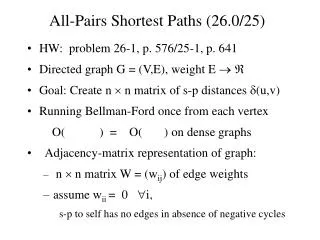
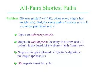
2. Dynamic All Pairs Shortest Paths Given a weighteddirectedgraph G=(V,E,w),perform any intermixed sequence of the following operations: update weight of edge (u,v) to w Update(u,v,w): return distance from x to y Distance(x,y): returnshortest pathfrom x to y Path(x,y):

3. ~ O(n3) King 99 general [0,C] O(n2.5 (C log n)0.5) O(1) Henzinger et al. 97 planar [0,C] O(n9/7 log(nC)) Fackcharoemphol, Rao 01 planar reals O(n9/5 log13/5 n) general reals ? < o(n3) O(1) D, Italiano 01 general S reals O(n2.5 (S log3 n)0.5) O(1) Previous work on fully dynamic APSP Graph Weight Update Query reals Update recomputingfrom scratch general O(1) ~ [0,C] O(n2.575 C0.681)

4. Contributions of This Paper • A completely new approach to dynamic APSP. • A fullydynamic algorithm for APSP on generaldirected graphs with nonnegative real-valued edge weights. • Supporting any sequence of operations in O(n2log3n) amortized time per update,unit worst-case time per distance query,and optimal worst-case time for returning any shortest path.

5. (n) (n) (n2) changes per update +1 -1 +1

6. A new approach New combinatorial properties of graphs: Locally shortest paths Uniform paths

7. x y πxy Shortest path Shortest path Not a shortest path Shortest path x y πxy Definition of Locally shortest paths • A path πxyis locally shortest in G if either: • πxyconsists of a single vertex, or • every proper subpath of πxyis a shortest path in G Locally Shortest NOT Locally Shortest

8. Locally shortest path Shortest path Shortest path Shortest path Properties of Locally shortest paths • In a locally shortest path, all proper subpaths are shortest paths: however, the path itself may not necessarily be shortest. u v y πxy x

9. Properties of Locally shortest paths Theorem I Shortest paths  Locally shortest paths Shortest paths Locally shortest paths

10. For the sake of simplicity, we assume that no two paths in the graph have the same weight. π1 π2 x y π3 Properties of Locally shortest paths (Ties can be broken by adding a tiny fraction to the weight of each edge) Theorem II Locally shortest paths πxy are internally vertex-disjoint

11. x y Properties of Locally shortest paths Theorem III There are at most n-1 Locally shortest paths connecting x,y This is a consequence of vertex-disjointess…

12. ≤ mchoices ≤ nchoices Properties of Locally shortest paths Theorem IV If shortest paths are unique in G, then there can be at mostm·n locally shortest paths in G. y x v ≤mn ×

13. We call dynamic graph a sequence of graphs <G0,…,Gk> such that, for any t, Gt-1and Gt differ in the weight of exactly one edge, 0≤t≤k. Dynamic graphs

14. p v u Gt-1 x y q u p v Gt x y q Locally shortest paths in dynamic graphs An Locally shortest path in Gt is appearing if it is not Locally shortest in Gt-1

15. u p v Gt x y q u p v A Locally shortest path in Gt is disappearing if it is not Locally shortest in Gt+1 Gt+1 x y q Locally shortest paths in dynamic graphs

16. Locally shortest paths in dynamic graphs Proof • A path can stop being locally shortest only if any of its proper subpaths stops being shortest. • In case of increases, this can happen only if the subpath contains the updated vertex, say vertex v. • By theorem II, at most O(n2) shortest paths contain v as an internal vertex. • At most O(n2) locally shortest paths starting or ending at v. Theorem V Let G be a graph subject to a sequence of vertex updates. If shortest paths are unique in G, then in the worst case at most O(n2) paths can stop being locally shortest due to a vertex increase.

17. Locally shortest paths in dynamic graphs Theorem VI • Let G be a graph subject to a sequence Σof increase-only vertex updates and let m be the maximum number of edges in G throughout the sequence Σ. If shortest paths are unique in G, then the number of paths that start being locally shortest after each update is: • O(mn) in the worst case. • O(n2) amortized over Ω(m/n) updates. Proof of (2) • Assume that initially there are x0 locally shortest paths. x0 = O(mn). • Assume that there are k updates, k≥m/n. By Theorem V, O(k n2) paths can stop being locally shortest. • xk ≤ mn. • Assume the total number of paths that start being locally shortest is y. • x0 - O(k n2)+ y ≤ xk y ≤ O(k n2)+ xk- x0 = O(k n2) + O(mn)-O(mn)= O(k n2) + O(mn)= O(k n2)y/k ≤ O(n2)

18. What about fully dynamic sequences? 10 10 20 20 x x y y 100 30 30 40 40 Locally shortest paths in dynamic graphs The weights of Locally shortest paths that disappear and then reappear do not change…

19. The shortest path is the same, but has different weight: EASY EASY x y  The shortest path is different (update = decrease): x y - Shortest paths and edge weight updates How does a shortest path change after an update?

20. a b + HARD The shortest path is different (update = increase): If we look closer, we realize that the new shortest path from a to b was already Locally shortest before the update! x y Shortest paths and edge weight updates

21. For each pair x,y, maintain in a data structure Locally shortest pathsconnecting x to y Main idea: The combinatorial properties of Locally shortest paths imply that only a small piece of information needs to be updated at each time… Are we done? A new approach to dynamic APSP NO

22. x x y y x y This path stays the same while flipping between Locally shortest and non-Locally shortest: We would like to have an update algorithm that pays only once for it over the whole sequence... How to pay only once?

23. may x y resurrect! x y This path remains a shortest path after the insertion This path is no longer a shortest path after the insertion… Looking at the substructure …but if we removed the edge it would get a shortest path again!

24. Breaking Ties • If shortest paths in the graph are not unique, the properties of locally shortest paths don’t hold. • Using an arbitrary tie-breaking strategy may lead to incorrect results.

25. Breaking Ties – Basic idea • Without loss of generality, assume that V = {1, 2, …, n}. • Assign to each edge (u, v) a unique number ID(u, v) (e.g. ID(u, v)=u+nv). • For each path π, define ID(π) as the maximum ID of its edges. • For a path π , extended weight ew(π) = (w(π), ID(π)).

26. Breaking Ties – Comparing two ew’s Compare the extended weights of two paths π1 and π2 • ew(π1) ≤ ew(π2) if and only if • w(π1) < w(π2)or • w(π1) = w(π2)and ID(π1)≤ ID(π2).

27. Breaking Ties Definition of Sew Let G be a graph with real-valued edge weights and let ew be the extended weight function. We define Sew as follows: Note:Sew contains every path in G that has minimum extended weight and whose subpaths have minimum extended weight as well.

28. Lemma I For each pair of vertices x and y in G, there can be at most one path connecting them. Lemma II For each pair of vertices x and y in G, there is a path . Breaking Ties • Sew contains exactly one shortest path between each pair of vertices connected in G. • |Sew| ≤ n2. • Sew is a complete set of unique shortest paths in G. • We can always ensure uniqueness of shortest paths by dealing with paths in Sew.

29. Historical paths Definition of Historical paths Let πxy be a path in G at time t, and let t’ ≤ t be the time of the latest vertex update on πxy. We say that πxy is HISTORICAL at time t if it has been a shortest path at least once in the time interval [t’, t]. Note:A shortest path is also a historical path. Although it may stop being a shortest path at some point, it keeps on being a historical path until a vertex update occurs on it.

30. Locally historical paths Definition of Locally historical paths • We say that a path πxy is Locally Historical in G at time t if either: • πxy consists of a single vertex, or • Every proper subpath of πxy is a historical path in G at time t.

31. shortest path x Locally shortest path πxy y shortest path shortest or historical path x Locally historical path πxy y shortest or historical path Locally historical paths vs. Locally shortest paths Relaxed notion of Locally historical: Subpaths do not need to be shortest at the same time

32. Theorem Locally shortest paths  Locally historical paths Shortest paths Properties of Locally historical paths Locally historical paths Locally shortest paths

33. Properties of Locally historical paths Theorem (Assume there are at most z historical paths between each pair of vertices) O(zn2) historical paths at any time O(zn2) new Locally historical paths per update

34. A lot! We can construct a dynamic graph with (n3) historical paths at any time, amortized. 100 100 100 (n) (n) 90 90 100 90 80 80 (n) 70 = (n3) # h paths = (n2) +(n2) +(n2) (n) How many historical paths can we have?

35. 100 90 100 90 80 100 100 100 100 70 100 100 (n) (n) 90 90 90 90 100 90 90 80 80 80 80 (n) 70 70 (n2) (n2) (n2) 0 (in general, O(n2)) Reducing # of historical paths: Smoothing At each update we pick an edge with the maximum number of historical paths passing through it, and we remove and reinsert it # h paths =

36. For each pair x,y, maintain in a data structure the Locally historical paths connecting x to y Main idea: The combinatorial properties of Locally historical paths imply that, if we do smoothing, we have only O(n2) new Locally historical paths per update, amortized… A new approach to dynamic APSP (II)

37. EASY + The shortest path is different (update = increase): If we maintain Locally historical paths using priority queues, we can find this path in O(1) time! x y Handling the hard case

38. Remove from the data structure all Locally historical paths containing the updated edge 1 Use remaining Locally historical paths to find an upper bound to the distances after the update 2 Propagate changes in waves from the updated edge, finding the new Locally historical paths and the new distances 3 The update algorithm

39. Locally historical paths are the heart of dynamic shortest paths O(n2 log3 n) amortized time per fully-update operation Distance and path query in optimal time. Conclusions

40. Homework – 4 Formulate a practical problem as a fully dynamic all pairs shortest paths problem. (please don’t use railway or highway systems as examples.)