Download

1 / 43
430 likes | 626 Vues
Learn about dynamic programming, comparing to divide-and-conquer, and solving the all-pairs shortest paths problem efficiently. Dive into algorithms like Floyd-Warshall and matrix multiplication in this comprehensive guide.

E N D
Dynamic programming • Comparing to divide-and-conquer • Both partition the problem into sub-problems • Divide-and-conquer partition problems into independent sub-problems, dynamic programming is applicable when the sub-problems are dependent.
Dynamic programming • Comparing to greedy method: • Both are applicable when a problem exhibits optimal substructure • In greedy algorithms, we use optimal substructure in a top-down fashion, that is, without finding optimal solutions to sub-problems, we first make a choice that looks best at the time-and then solve a resulting sub-problem. While in dynamic programming, we use optimal substructure in a bottom-up fashion, that is, we first find optimal solutions to sub-problems and, having solved the sub-problems, we find an optimal solution to the problem.
Dynamic programming • The development of a dynamic programming algorithm can be broken into four steps: • Characterize the structure of an optimal solution. • Recursively define the value of an optimal solution. • Compute the value of an optimal solution in a bottom-up fashion. • Construct an optimal solution from computed information. Steps 1-3 form the basis of a dynamic-programming solution to a problem. Step 4 can be omitted if only the value of an optimal solution is required. When we do perform step 4, we sometimes maintain additional information during the computation in step 3 to ease the construction of an optimal solution.
0-1 version v/w: 1, 3, 3.6, 3.66, 4.
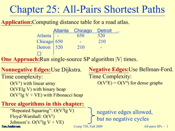
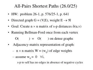
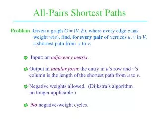
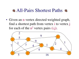
All –pairs shortest-paths problem • Problem: Given a directed graph G=(V, E), and a weight function w: ER, for each pair of vertices u, v, compute the shortest path weight (u, v), and a shortest path if exists. • Output: • A VV matrix D = (dij), where, dij contains the shortest path weight from vertex i to vertex j. //Important! • A VV matrix =(ij), where, ij is NIL if either i=j or there is no path from i to j, otherwise ij is the predecessor of j on some shortest path from i. // Not covered in class, but in Exercises!
Methods • Application of single-source shortest-path algorithms • Direct methods to solve the problem: • Matrix multiplication • Floyd-Warshall algorithm • Johnson’s algorithm for sparse graphs • Transitive closure (Floyd-Warshall algorithm)
Matrix multiplication--suppose there are no negative cycles. • A dynamic programming method: • Study structure of an optimal solution • Solve the problem recursively • Compute the value of an optimal solution in a bottom-up manner • The operation of each loop is like matrix multiplication.
Matrix multiplication—structure of a shortest path • Suppose W = (wij) is the adjacency matrix such that Consider a shortest path P from i to j, and suppose that P has at most m edges. Then, if i = j, P has weight 0 and no edges. If i j, we can decompose P into ikj, P’ is a shortest path from i to k. P’
Matrix multiplication—recursive solution Let lij(m) be the minimum weight of any path from i to j that contains at mostm edges. • lij(0) = 0, if i = j, and otherwise. • For m 1, • lij(m) = min{lik(m-1)+wkj}, 1 k n • The solution is lij(n-1)
Matrix Multiplication • Solve the problem stage by stage (dynamic programming) • L(1) = W • L(2) • … • L(n-1) • where L(m), contains the shortest path weight with path length m.
Matrix multiplication (running time) • O(n4) Improving the running time: • No need to compute all the L(m) matrices for 1 m n-1. We are interested only in L(n-1), which is equal to L(m) for all integers m ≥ n-1, with assuming that there are no negative cycles.
Improving the running time Compute the sequence L(1) = W, L(2) = W2 = WW , L(4) = W4 = W2W2, L(8) = W8 = W4W4 ... We need only lg(n-1) matrix products • Time complexity: O(n3 lg n)
Floyd-Warshall algorithm--suppose there are no negative cycles.-structure of shortest path
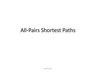
Floyd-Warshall algorithm(idea) • dij(k): shortest path weight from i to j with intermediate vertices (excluding i, j) from the set {1,2,…,k} • Intermediate vertex of a simple path p = <v1, v2, …, vl> is any vertex of pother thanv1 or vl. • dij(0) = wij (no intermediate vertices at all) • How to compute dij(k) from D(r), for r < k?
Floyd-Warshall algorithm-recursive solution • dij(0) = wij (no intermediate vertices at all) dij(k) = min(dij(k-1), dik(k-1) + dkj(k-1)) if k ≥ 1 Result: D(n) = (dij(n)) (because all intermediate vertices are in the set {1, 2, …, n})
Floyd-Warshall algorithm-compute shortest-path weights • Solve the problem stage by stage: • D(0) • D(1) • D(2) • … • D(n) • where D(k) contains the shortest path weight with all the intermediate vertices from set {1,2…,k}.
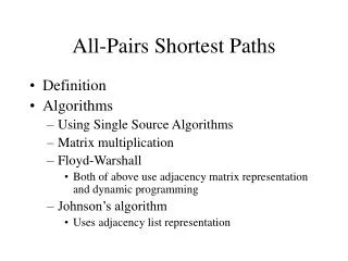
Floyd-Warshall algorithm 2 k=1: d43(1)=-5; d42(1)=5; d45(1)=-2 4 3 1 3 8 2 -4 1 -5 7 5 4 6
Floyd-Warshall algorithm 2 k=2: d43(2) =-5; d42(2)=5; d45(2)= 2 4 3 1 3 8 2 -4 1 -5 7 5 4 6
Floyd-Warshall algorithm 2 k=3: d42(3)=-1; d43(3)=-5; d45(3)=-2 4 3 1 3 8 2 -4 1 -5 7 5 4 6
Floyd-Warhsall algorithm (pseudo-code) Time complexity: O(n3) Space: O(n3)
Floyd-Warshall algorithm(less space) Notice that: we can write dij(k) directly on D(k-1) k-th column dij(k) dik(k-1) dkj(k) dkj(k-1) k-th row dik(k) dij(k)
Constructing a shortest path • For k = 0 • For k 1
2 4 3 1 3 8 1 -5 -4 2 7 5 4 6 Example:
D(0)= (0)= (1)= D(1)=
D(2)= (2)= D(3)= (3)=
D(4)= (4)= (5)= D(5)=
Shortest path from 1 to 2 in 2 4 3 1 3 8 1 -5 -4 2 7 5 4 6
Transitive closure (the problem) • Given a graph G=(V, E), compute the transitive closure G* = (V, E*), where E* = {(i, j): There is a path from i to j in G} a c b i j
Transitive closure • One way: set wij = 1 and run the Floyd-Warshall algorithm, if dij(n) <, then (i, j) E* • Running time O(n3)
transitive closure • Another way: Substitute “+” and “min” by AND and OR in Floyd’s algorithm • Running time O(n3)