All-Pairs Shortest Paths

1. All-Pairs Shortest Paths • Definition • Algorithms • Using Single Source Algorithms • Matrix multiplication • Floyd-Warshall • Both of above use adjacency matrix representation and dynamic programming • Johnson’s algorithm • Uses adjacency list representation

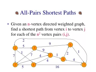
2. Definition • Input • Weighted, connected directed graph G=(V,E) • Weight (length) function w on each edge e in E • We will typically assume w is represented as a matrix • Task • Compute a shortest path from all nodes in V to all nodes in V • Still have issue with negative weight cycles

3. Using single source algorithms • Call a single source algorithm from each vertex s in V • O(V X) where X is the running time of the given algorithm • Dijkstra linear array: O(V3) • Dijkstra binary heap: O(VE log V) • Dijkstra Fibonacci heap: O(V2 log V + VE) • Bellman-Ford: O(V2 E) (negative weight edges)

4. Two adjacency matrix based algorithms • Matrix-multiplication based algorithm • Let Lm(i,j) denote the length of the shortest path from node i to node j using at most m edges • What is our desired result in terms of Lm(i,j)? • What is a recurrence relation for Lm(i,j)? • Floyd-Warshall algorithm • Let Lk(i,j) denote the length of the shortest path from node i to node j using only nodes within {1, …, k} as internal nodes. • What is our desired result in terms of Lk(i,j)? • What is a recurrence relation for Lk(i,j)?

5. Conceptual pictures Shortest path using at most 2m edges Try all possible nodes k i k j Shortest path using at most m edges Shortest path using at most m edges Shortest path using nodes 1 through k Shortest path using nodes 1 through k-1 i k j Shortest path using nodes 1 through k-1 OR Shortest path using nodes 1 through k-1

6. Running Times • Matrix-multiplication based algorithm • O(V3 log V) • log V executions of “matrix-matrix” multiplication • Not quite matrix-matrix multiplication but same running time • Floyd-Warshall algorithm • O(V3) • V iterations of an O(V2) update loop • The constant is very small, so this is a “fast” O(V3)

7. Johnson’s Algorithm • Key ideas • Reweight edge weights to eliminate negative weight edges AND preserve shortest paths • Use Bellman-Ford and Dijkstra’s algorithms as subroutines • Running time: O(V2 log V + VE) • Better than earlier algorithms for sparse graphs

8. Reweighting • Original edge weight is w(u,v) • New edge weight: • w’(u,v) = w(u,v) + h(u) – h(v) • h(v) is a function mapping vertices to real numbers • Key observation: • Let p be any path from node u to node v • w’(p) = w(p) + h(u) – h(v)

9. Computing vertex weights h(v) • Create a new graph G’ = (V’, E’) by • adding a new vertex s to V • adding edges (s,v) for all v in V • w(s,v) = 0 for all v in V • Set h(v) to be the length of the shortest path from this new node s to node v • This is well-defined if G’ does not contain negative weight cycles • Note that h(v) <= h(u) + w(u,v) for all (u,v) in E’ • Thus, w’(u,v) = w(u,v) + h(u) – h(v) >= 0

10. Algorithm implementation • Run Bellman-Ford on G’ from new node s • If no negative weight cycle, then use h(v) values from Bellman-Ford • Now compute w’(u,v) for each edge (u,v) in E • Now run Dijkstra’s algorithm using w’ • Use each node as source node • Modify d[u,v] at end by adding h(v) and subtracting h(u) to get true path weight • Running time: • O(VE) [from one run of Bellman-Ford] + • O(V2 log V + VE) [from V runs of Dijkstra]