Download
1 / 49
500 likes | 796 Vues
Nonlinear Dynamics of Iterative Decoding Systems: Analysis and Applications . Ljupco Kocarev University of California, San Diego. Summary of the presentation. Nonlinear Dynamics of the iterative coding systems Nonlinear Codes with Latin Squares (Quasi-groups) Conclusions .

E N D
Nonlinear Dynamics of Iterative Decoding Systems: Analysis and Applications Ljupco Kocarev University of California, San Diego
Summary of the presentation • Nonlinear Dynamics of the iterative coding systems • Nonlinear Codes with Latin Squares (Quasi-groups) • Conclusions
When: since 2002 Who: Alex Vardy (UCSD) Gian Mario Maggio (ST, Swiss) Zarko Tasev (Kyocera, USA) Frederic Lehmann (INT, Paris, France) Pater Popovski (Tech University, Denmark) Bartolo Scanavino (Poli Torino, Italy) • Why: • To understand finite-length iterative decoding algorithms using tools from nonlinear systems and chaos theory; and • To exploit chaos theory for enhancing existing iterative coding techniques and invent new classes of error-correcting codes. Sponsors: ARO (MURI), STMicroelectronics, University of California (DIMI)
Understanding finite-length iterative coding systems As of today asymptotic behavior (as the block-length tends to infinity) of iterative coding systems is reasonably well understood • Codes on graphs as spin models (1989) • Finite length scaling for iterative coding systems (2004) • Renormalization group approach for iterative coding systems (2003) • Scale-free networks and error-correction code (2004) • Nonlinear dynamics of iterative coding systems (2000) Tom Richardson: The geometry of turbo decoding dynamics (2000)
1/2 1/3 1/2 0 1 01 2/3 00 Kalman’s example R. E. Kalman, 1956 “Nonlinear aspects of sampled-data control systems” xn+1 1 Markov process with transition probabilities: 1 S 1/3 0 xn 0 1/3 2/3 1 1 0 S Logistic map: xn+1 = a xn ( 1 – xn ) a = 3.839
Turbo codes n=1024 Classical turbo codes: C. Berrou, A Glavieux, and P. Thitimajshima, “Near Shannon limit error-correcting coding and decoding: Turbo-Codes,” Proc. IEEE International Communications Conference, pp. 1064-70, 1993
Turbo-decoding algorithm AWGN channel BCJR algorithm, 1974 X1, X2 - extrinsic information exchanged by the two SISO decoders c0, c1, c2 - channel outputs corresponding to the input sequences
The system depends smoothly on its 2n variables X1, X2 and 3n parameters c0, c1, c2 (Richardson) E represents a posteriori average entropy Three types of plots: E(l) versus l, E(l+1) versus E(l), and E versus SNR.
Discrete-time Hopf bifurcation (part I) -6.7dB -6.5dB -6.3dB -6.1dB 0.75dB 0.8dB 0.85dB -5.9dB
Discrete-time Hopf bifurcation (part II) -6.7dB -6.6dB -6.5dB -6.3dB -6.2dB -6.1dB
Example: 2D map a = 1.9, 2.1, 2.16, 2.27 • Attracting fixed point • Attracting invariant curve • Chaotic attractor
Tangent bifurcation (part I) -7.65dB -7.645dB -7.6dB 0.3dB 0.35dB 0.4dB
Tangent bifurcation (part II) -7.65dB -7.65dB -7.64dB -7.64dB
Transient chaos • The unequivocal fixed point • becomes stable around –1.5dB. • Region 0.25dB to 1.25dB • (waterfall region): transient chaos • Average chaotic transient lifetime • for SNR=0.8dB is 378 iteration
Transient chaos For each SNR, we generate 1000 different noise realizations (1000 different parameters frames) and compute the number of decoding trajectories that approach the fixed point in less than a given number of iterations. At SNR of 0.6dB, there are 492 frames that converge to the unequivocal fixed point in 5 or less iterations, another 226 frames converge in 10 or less iterations, and so on, while 58 frames remain chaotic after 2000 iterations (which means that their trajectory either approaches a chaotic attractor or that the transient chaos lifetime is very large).
LDPC codes Torus-breakdown route to chaos for the regular (216,3,6) LDPC code The values of SNR corresponding to the invariant sets, starting from the fixed point towards chaos, are: 1.19 dB, 1.23 dB, 1.27 dB, 1.33 dB, and 1.44 dB
Control of transient chaos Average chaotic transient lifetime for SNR=0.8dB is 9 iterations.
Conclusions • Iterative decoding algorithms can be viewed as high-dimensional dynamical systems parameterized by a large number of parameters. However, although the iterative-decoding algorithm is a high-dimensional dynamical system, it apparently has only a few active variables. • The waterfall region for all iterative coding systems exhibits reach dynamical behavior: chaotic attractors, transient chaos, multiple attractors and fractal basin boundaries. • Applications: • We have proposed a simple adaptive technique to control transient chaos in the turbo decoding algorithm. This results in a ultra-fast convergence and a significant gain in terms of BER performance. • We have proposed a novel stopping criterion for turbo codes based on the average entropy of an information block. This is shown to reduce the average number of iterations and to benefit from the use of the adaptive control technique.
Open problems: • Study how the size of the basin of attraction changes with varying SNR. • Find how the value of SNR for which the fixed point at origin becomes a stable point related to the threshold which gives the boundary of the error-free region. • Study whether the chaotic behavior of the iterative coding systems comes from the presence of cycles in the graph. • Investigate how the topological structure of unstable periodic orbits embedded into the chaotic set is related to the topological structure of the factor graph. • Use ergodic theory for dynamical systems to study the properties related to a set of trajectories, not a single trajectory. • Find models of low-dimensional dynamical systems averaged over ensembles and/or different noise realizations.
Latin Squares (Quasigroups) D. Gligoroski, S. Markovski (since Sep 2004) A Latin square of order N is NxN array of numbers from N-symbol alphabet (say 0, 1, 2, … N-1) in which each row and each column contains each symbol exactly once. Latin squares are also linked to algebraic objects known as quasigroups. A quasigroup is defined in terms of a set, Q, of distinct symbols and a binary operation (called multiplication) involving only the elements of Q. A quasigroup's multiplication table turns out to be a Latin square.
Given a quasigroup (Q,*) five new operations, so called parastrophes or adjoint operations, can be derived from the operation *. We need only the following one defined by: (Q,\) is also a quasigroup.
Quasigroup string transformations e-transformation d-transformation
Let Q+ be the set of all nonempty words (i.e. finite strings) formed by the elements of Q.
Nonlinear Codes with Latin Squares (Quasigroups) (Q,*) Q = {0, 1, 2, … N-1} M1, M2, …, Mr information string; each Mi is an element of Q L1, L2, …, Lm m> r Each Li is either Mi or 0 C1, C2, …, Cm codeword
k1, k2, …, kn leaders each ki is an element of Q
Properties of the Code • Nonlinear code • “Almost random” code • C1, C2, ?, C3, …, CmL1, L2, ?, ?, …., ? • (synchronous and self - synchronized stream ciphers)
Example (Q,*) Q = {0, 1, 2, … 15} Quasigroup of order 16 Each Mi is a nibble (4-bit string)
Decoding the code BSC Di is a nibble and D(i) is a sub-block of 4 nibbles (16 bits)
If the set Ss contains only one element we say the decoding is successful
Stability of the decoding algorithm Theorem: If the decoding is successful, then the message is recovered with probability 2-N(1-R) Conjecture: If then the decoding procedure converges and the cardinality of Ss is 1. The relative Gilbert-Varshamov (GV) distance
Example • Reed – Muller code (6,32) rate 3/16 corrects up to 7 errors • Total number of noisy code-words the codes can correct is 4.5 x 10⁶ m1 m2 02 02 02 02 02 02 m3 02 02 02 02 02 02 02 (6,32) rate 3/16 N = 32 Bmax = 8 (B2 = 8) Bmax = 5 68852 ~ 4.7 107
Conclusions (open problems) • Theoretical framework • AWGN channel, soft decoding • Concatenated codes: Si is intersection of two sets Si(1) and Si(2)