Download

1 / 61
610 likes | 625 Vues
PRESIDENCY UNIVERISTY, BENGALURU School of Engineering Computer Organization and Architecture CSE205 IV Semester 2018-19. Module 4. Arithmetic Unit. A basic operation in all digital computers is the addition or subtraction of two numbers.

E N D
PRESIDENCY UNIVERISTY, BENGALURU School of Engineering Computer Organization and Architecture CSE205 IV Semester 2018-19
Module 4 Arithmetic Unit
A basic operation in all digital computers is the addition or subtraction of two numbers. In this chapter we discuss about the logic circuits used to implement arithmetic operations. The time needed to perform an addition operation affects the processor’s performance. Multiply and divide operations, which require more complex circuitry than either addition or subtraction operations, also affect the performance. In this chapter we discuss about some of the techniques used in modern computers to perform arithmetic operations at high speed. Compared with arithmetic operations, logic operations are simple to implement using combinational circuits. Introduction
Consider the addition of two numbers X and Y with n-bits each. Figure 6.1 shows the logic truth table for adding equally weighted bits Xi and Yi intwo numbers X And Y. The figure also shows the logic expressions for these functions, along with an example of addition of 4-bit unsigned numbers 7 and 6. The logic expression for sum (Si) and the carry out function (Ci+1) are shown in the figure. Addition And Subtraction Of Two Numbers
FULL ADDER: The circuit which performs the addition of three bits is a Full Adder. It consists of three inputs and two outputs. INPUTS: Xi, yi and ci are the three inputs of full adder. OUTPUTS: Si and Ci+1 are the two outputs of full adder. Block diagram of full adder is shown in the figure. A cascaded connection of n full adder blocks can be used to add two n-bit numbers. Since the carries must propagate or ripple through this cascade, the configuration is called an n-bit ripple-carry adder. A cascaded connection of K n-bit adders can be used to add k n-bit numbers.
Computing the add time (contd..) y0 x0 FA c1 c0 s0 Consider 0th stage: • c1 is available after 2 gate delays. • s0 is available after 1 gate delay. Carry Sum y i c i x i x i c y s c i i i + 1 i c i x i y i
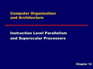
y0 x0 y0 x0 y0 y0 x0 x0 FA FA FA FA c0 c1 c2 c3 c4 s0 s1 s3 s2 Computing the add time (contd..) Cascade of 4 Full Adders, or a 4-bit adder • s0 available after 1 gate delays, c1 available after 2 gate delays. • s1 available after 3 gate delays, c2 available after 4 gate delays. • s2 available after 5 gate delays, c3 available after 6 gate delays. • s3 available after 7 gate delays, c4 available after 8 gate delays. For an n-bit adder,sn-1is available after 2n-1 gate delays cnis available after2ngate delays.
Fast addition (Carry-look Ahead Addition) Recall the equations: Second equation can be written as: We can write: • Giis called generate function andPiis called propagate function • Gi and Pi are computed only from xiand yi and not ci, thus they can • be computed in one gate delay after X and Y are applied to the • inputs of an n-bit adder.
The expressions Giand Piare called the generate and propagate functions for stage i. Each bit stage contains an 1) AND gate to form Gi, 2)OR gate to form Pi, and 3)three-input XOR gate to form Si. A simpler circuit can be designed to generate Gi, Si and Pi But in this case Gi=1, so it does not matter whether Pi is 0 or 1. Then using a cascade of two input XOR gates to realize the 3-input XOR function. the basic cell B can be used in each bit stage as shown in the figure.
For example the carries in a four stage carry-look ahead adder is given as follows. C1= G0+P0C0 C2=G1+P1C1 = G1+ P1(G0+P0C0) = G1+P1G0+P1P0C0 C3= G2+P2C2 = G2+P2(G1+P1G0+P1P0C0) = G2+P2G1+P2P1G0+P2P1P0C0
C4= G3+P3C3 = G3+P3(G2+P2G1+P2P1G0+P2P1P0C0) = G3+P3G2+P3P2G1+P3P2P1G0+P3P2P1P0C0 Higher-level generate and propagate Functions: P0I=P3P2P1P0 G0I=G3+P3G2+P3P2G1+P3P2P1G0
Pi and Gi: All Pi and Gi are available after one gate delay. Ci+1: All carries are available after three gate delays. Sum: After a further XOR gate delay, all sum bits are available. So after four gate delays all sums are available.
The complete 4-bit adder is shown in the figure 6.4b An adder implemented in this form is called a carry-look ahead adder. Delay through the adder is 3gate delays for all carry bits and 4 gate delays for all sum bits. In comparison 4-bit ripple carry adder requires 7 gate delays for all sums and 8 gate delays for all carries. If we cascade a number of 4-bit adders as shown in the figure 6.2c it is possible to built longer adders.
Eight four-bit carry look-ahead adders can be connected to form a 32-bit adder. Gate Delays for all carries and sums are calculated as follows: The carry out C4 from the low-order 4-bit adder is available after 3 gate delays. The C8 is available at the output of the second adder after a further 2 gate delays, C12 is available after further 2 gate delays and soon. Finally C28 is available after a total of (6*2)+3= 15 gate delays. Then c32 and all carries inside the high-order adder are available after a further 2 gate delays.
All carries are available after 17 gate delays All 4 sum bits are available after 1 more gate delay, for a total of 18 gate delays. In the next section, we discuss how to generate the carries C4, C8, and C12 ............. in parallel, similar to the way that C1,C2, C3 and C4 are generated in parallel in the 4-bit carry-look ahead adder. Higher level generate and propagate functions: In 32-bit adder just discussed, the carries C4,C8,C12……… ripple through 4-bit adder blocks with two gate delays per block. By using higher level block generate and propagate functions, it is possible to use the look-ahead approach to develop the carries C4,C8,C12……… in parallel in a higher-level carry-look-ahead circuit.
The figure below shows a 16-bit adder built from four 4-bit adder block. These blocks provide new output functions defined as GKI and PKI where K=0 for the first 4-bit block. And K=1 for the second 4-bit block. In the first block P0I= P3P2P1P0 G0I= G3+P3G2+P3P2G1+P3P2P1G0 Where Gi and Pi are generate and propagate functions of bit stage I, GKI and PKIare generate propagate functions of block K 16-bit carry look-ahead adder built from four 4-bit adders
With these new functions available, it is not necessary to w for carries to ripple through the 4-bit blocks. Gi and Pi: Lower level generate and propagate functions are available after one gate delay. Gi=XiYi Pi= Xi+Yi GkI and PKI: two gate delays are needed to develop higher level propagate and generate functions.
C4,C8,C12,C16: C4= G0I+P0IC0 C8 = G1I+ P1IC4 = G1I+P1G0I+P1P0IC0 C12= G2I+P2IC8 = G2I+P2(G1I+P1G0I+P1P0IC0) = G2I+P2IG1I+P2IP1IG0I+P2IP1IP0IC0 C16= G3I+P3IC12 = G3I+P3I(G2I+P2IG1I+P2IP1IG0I+P2IP1IP0IC0) Two more gate delays are required to generate these carries
Two more gate delays are required to generate internal carries in each block 1st Block In first block internal carries are C5,C6,C7 C5=G4+P4C4 C6=G5+P5C5 =G5+P5(G4+P4C4) =G5+P5G4+P5C4 C7=G6+P6C6 =G6+P6(G5+P5G4+P5C4) =G6+P6G5+P6P5G4+P6P5C4 Two gate delays are needed to generate C5,C6,C7. Similarly to generate internal carries in 2nd block, 3rd block, and 4th block two gate delays are required.
Gate delays: Pi and Gi are available after 1 gate delay. Pki and Gki are available after 3 gate delays. External carries (C4,C8,C12,C16) are available after 5 gate delays. Internal carries are available after 7 gate delays. Hence all carries are available after 7 gate delays. So, one more gate delay is required to generate all sums. Hence all sums are available after 8 gate delays.
Signed-operand Multiplication • Considering 2’s-complement signed operands, what will happen to (-13)(+11) if following the same method of unsigned multiplication? 1 0 0 1 1 ( - 13 ) ( ) 0 1 0 1 1 + 11 1 1 1 1 1 1 0 0 1 1 1 1 1 1 1 0 0 1 1 Sign extension is 0 0 0 0 0 0 0 0 shown in blue 1 1 1 0 0 1 1 0 0 0 0 0 0 1 1 0 1 1 1 0 0 0 1 ( - 143 ) Sign extension of negative multiplicand.
The booth algorithm generates the 2n-bit product and treats both positive and negative 2’s complement n-bit operands uniformly. In general, in the booth scheme, -1 times the shifted multiplicand is selected when moving from 0 to 1, and +1 times the multiplicand is selected when moving from 1 to 0. Example: Recode the multiplier 101100 for Booth’s algorithm? Multiplier: 1 0 1 1 0 0 0 Recoded Multiplier: -1 +1 0 -1 0 0 ; Booth Algorithm
To speed-up the multiplication process in the Booth’s algorithm a technique called Bit-pair Recoding is used. It is also called modified algorithm. It halves the maximum number of summands. Fast Multiplication
Bit-Pair Recoding of Multipliers • Bit-pair recoding halves the maximum number of summands (versions of the multiplicand). Sign extension Implied 0 to right of LSB 1 1 1 0 1 0 0 1 2 0 (a) Example of bit-pair recoding derived from Booth recoding
The figure 6.20 shows the examples of decimal division and binary division of the same values. Integer Division Manual Division
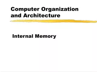
Circuit Arrangement Shift left qn-1 q0 Dividend Q A Quotient Setting N+1 bit adder Add/Subtract Control Sequencer m0 a0 mn-1 an-1 an 0 Divisor M Figure 6.21.Circuit arrangement for binary division.
Figure 6.21 shows a logic circuit arrangement that implements restoring division. An n-bit positive divisor is loaded into register M. An n-bit positive dividend is loaded into register Q at the start of the operation. Register A is set to 0. After the division is complete, n-bit Quotient Register Q Remainder Register A The extra bit position at the end of both A and M accommodates the sign bit during subtractions. Restoring Division
The following algorithm performs the restoring division: Do the following ‘n’ times: Shift A and Q left one binary position. Subtract M from A, and place the answer back in A. If the sign of A is 1, set Q0 to 0 and add M back to A(that is, restore A); otherwise set Q0 to 1. Figure 6.22 shows a 4-bit example as it would be processed by the circuit in the figure 6.21 Restoring Division
1 0 Examples 1 1 1 0 0 0 1 1 1 1 0 Initially 0 0 0 0 0 1 0 0 0 0 0 0 1 1 Shift 0 0 0 0 1 0 0 0 Subtract 1 1 1 0 1 First cycle Set q 1 1 1 1 0 0 Restore 1 1 0 0 0 0 1 0 0 0 0 Shift 0 0 0 1 0 0 0 0 Subtract 1 1 1 0 1 Second cycle Set q 1 1 1 1 1 0 Restore 1 1 0 0 0 1 0 0 0 0 0 Shift 0 0 1 0 0 0 0 0 Subtract 1 1 1 0 1 q Third cycle Set 0 0 0 0 1 0 Shift 0 0 0 1 0 0 0 0 1 Subtract 1 1 1 0 1 0 0 1 Set q 1 1 1 1 1 0 Fourth cycle Restore 1 1 0 0 0 1 0 0 0 1 0 Remainder Quotient Figure 6.22:A restoring-division example.
Non restoring Division • Avoid the need for restoring A. • Any idea? • Step 1: (Repeat n times) • If the sign of A is 0, shift A and Q left one bit position and subtract M from A; otherwise, shift A andQleft and add M toA. • Now, if the sign of A is 0, set Q0 to 1; otherwise, set Q0 to 0. • Step2: If the sign of A is 1, add M to A
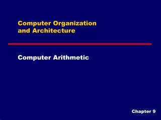
Examples Initially 0 0 0 0 0 1 0 0 0 0 0 0 1 1 Shift 0 0 0 0 1 0 0 0 First cycle Subtract 1 1 1 0 1 q Set 1 1 1 1 0 0 0 0 0 0 Shift 1 1 1 0 0 0 0 0 Add 0 0 0 1 1 Second cycle Set q 1 1 1 1 1 0 0 0 0 0 Shift 1 1 1 1 0 0 0 0 Add 0 0 0 1 1 Third cycle Restore remainder Set q 0 0 0 0 1 0 0 0 1 0 1 1 1 1 1 Add 0 0 0 1 1 Shift 0 0 0 1 0 0 0 1 0 0 0 1 0 Subtract 1 1 1 0 1 Fourth cycle Remainder Set q 1 1 1 1 1 0 0 1 0 0 Quotient A nonrestoring-division example.
Until now, we have discussed numbers without any decimal point, fixed point numbers. The decimal point is always assumed to be to the right of the least significant digit. e.g. 4.0 , 12.0, 24.0 (fixed-point numbers) Floating point numbers: The numbers in which the position of the decimal point is variable, such numbers are called Floating –point numbers. e.g. 0.25, 12.5, 323.865 Floating point numbers
Fixed point representation: It has limitations. Very large numbers cannot be represented, nor can very small fractions. e.g. 1) 976,000,000,000,000.000 2) 0.0000000000000976 Floating-point representation: The number 976,000,000,000,000.000 can be represented as 9.76 * 1014 Similarlythe fraction 0.0000000000000976 can be represented as 9.76*10-14 What we have done, we moved the decimal point to convenient location and use the exponent of 10 to indicate the position of decimal point. when decimal point is placed to the right of first (non zero) significant digit, the number is said to be normalized. This allows a range of very large and very small numbers to be represented with only a few digits.
The same approach can be taken with binary numbers. e.g. +111101.1000110 let us see how this number can be represented in the floating point format. +1.111011000110*25 (Normalized form) Floating point representation has three fields 1. sign 2. significant digits (mantissa) 3. Exponent In the above example sign = 0 mantissa = 11101100110 Exponent = 5
IEEE Standards For Floating- Point Numbers • The Standards for representing floating-point numbers in 32-bits and 64-bits have been developed by the Institute of Electrical and Electronics Engineers (IEEE). Single Precision: • The 32-bit standard representation of floating point numbers is called a Single-Precision representation. Sign: • The sign of the number is given in the first bit. • For positive numbers the sign bit is 0 and for negative numbers it is 1. Exponent: • Exponent field contains the representation for the exponent( to the base 2) of the scale factor. • Instead of the signed exponent, E, the value actually stored in the exponent field is an unsigned integer E΄ = E+127. • This is called Excess-127 format.
Thus E΄is in the range 0 ≤ E΄≤ 255. The end values of this range 0 and 255 are used to represent special values. Therefore the range of E΄ for normal numbers is 1 ≤ E΄≤ 254. This means the actual exponent, E is in the range -126≤ E ≤ 127. Mantissa: The string of significant bits commonly called the mantissa. The last 23-bits in single-precision represents the Mantissa. Since the most significant bit of the mantissa is always equal to 1, this bit is not explicitly represented, it is assumed to be to the immediate left of the binary point. Hence the 23-bits stored in mantissa field actually represent the fractional part of the Mantissa, this bits are right to the binary point. The single-precision representation is shown in the figure below.
Double Precision: The 64-bit standard representation of floating point numbers is called a double-Precision representation. The double precision format has increased exponent and mantissa ranges. Sign: The sign of the number is given in the first bit. For positive numbers the sign bit is 0 and for negative numbers it is 1. Exponent: Exponent field contains the representation for the exponent( to the base 2) of the scale factor. Instead of the signed exponent, E, the value actually stored in the exponent field is an unsigned integer E΄ = E+1023. This is called Excess-1023 format.